<?xml version="1.0" encoding="utf-8"?><feed xmlns="http://www.w3.org/2005/Atom" ><generator uri="https://jekyllrb.com/" version="3.9.5">Jekyll</generator><link href="https://yanlin-duan.github.io/feed.xml" rel="self" type="application/atom+xml" /><link href="https://yanlin-duan.github.io/" rel="alternate" type="text/html" /><updated>2024-04-13T21:04:04+00:00</updated><id>https://yanlin-duan.github.io/feed.xml</id><title type="html">Alan Duan</title><subtitle>Thoughts, knowledge and experiences</subtitle><author><name>Alan Duan</name><email>duanyanl97@gmail.com</email></author><entry><title type="html">在我消失的十天里</title><link href="https://yanlin-duan.github.io/life/vipassana/" rel="alternate" type="text/html" title="在我消失的十天里" /><published>2024-04-13T00:00:00+00:00</published><updated>2024-04-13T00:00:00+00:00</updated><id>https://yanlin-duan.github.io/life/vipassana</id><content type="html" xml:base="https://yanlin-duan.github.io/life/vipassana/"><![CDATA[<h1 id="引子">引子</h1>

<p>断网。</p>

<p>吃素。</p>

<p>禁酒。</p>

<p>禁欲。</p>

<p>住集体宿舍。</p>

<p>没有手机、书本、音乐、纸笔。</p>

<p>不能说话、对视。</p>

<p>不能与外界联系。</p>

<p>十天，每天四点起床，打坐冥想十小时。</p>

<p>唯一的好处？完全免费。</p>

<p>Vipassana 冥想营首先把它最骇人的一面毫无遮掩地展现在每一个申请者面前。即使如此，每年还是有上万人想来到这座“监狱”修行。课程需要提前好几个月报名，经常开放报名当天就满员。如果去油管、小红书或小宇宙上搜索，会找到很多博主说这是他们人生中最难、也最有收获的一段体验。</p>

<p>2023 年 10 月，我来到位于英国威尔士的 <a href="https://www.dhamma.org/en/schedules/schdipa">Dhamma Dipa</a> 中心，开始了我的十天“精神囚徒健身”。</p>

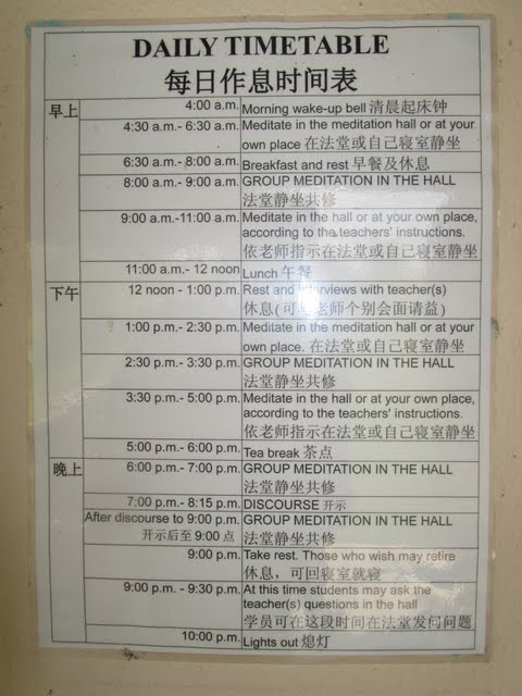
<table>
  <thead>
    <tr>
      <th style="text-align: center"><img src="https://yanlin-duan.github.io/assets/pics/vipassana/schedule.jpeg" alt="作息时间表。来自：https://jooiworld.com/posts/malaysia-vipassana.php" /></th>
    </tr>
  </thead>
  <tbody>
    <tr>
      <td style="text-align: center"><em>作息时间表。来自：https://jooiworld.com/posts/malaysia-vipassana.php</em></td>
    </tr>
  </tbody>
</table>

<h1 id="初探中心">初探中心</h1>

<p>先搭火车从伦敦到 Hereford，再从火车站坐约 45 分钟公交车。公交车翻过几座山头，在山中的一个小旅馆站下车。打电话让中心的司机来接。一辆红色 Honda 接上我，再在林间小道中开车约十分钟，直到开进一条车辆可以勉强通行的小路，才会看到位于深山老林中的 Dhamma Dipa。那阵子迷上读村上春树，感觉自己活像前去阿美寮看望直子的渡边。</p>

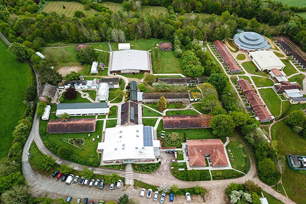
<p>中心挺大。从正门进入之后是办公区域和厨房，再往里便是食堂。从食堂开始便是对称的设计，左边是男区，右边是女区。再往里是居住区，男女区中间用墙或者挡板隔开，两侧分别有几座学生和志愿服务人员的宿舍。居住区往后走便是整座园区最核心的建筑，内观楼。楼内的设计又很简单，就是一片巨大的开放空间，可以供一百多人一起静坐冥想。开放空间的后面还有一些全黑的小隔间，供老生（上过至少一次十天课程的人）冥想使用。</p>

<p>内观楼背后则再次分隔成左右两片，这次不再是人工的分割，还是以树为界。男女两位助教（至于为什么是助教不是老师之后再讲）的宿舍就在树林入口处。这片树林可能是我最喜欢的地方了。初次进入，我不知道它会有多大，会通向哪里。我想起田村卡夫卡第一次进入小屋背后森林时的场景，想起大岛说不要让小屋离开你的视野的忠告。然而事实上，从入口走约几十步便能看到这片区域的主体样貌，是树围成的一片圆形草地。用闲庭信步的速度绕草地一周大概要三分钟。草地背后还有一片小树林，我管它叫后庭。草地的广阔视野和后庭郁郁葱葱的树林间形成了一种微妙的明暗对比。</p>

<p>我几次觉得在草地上站着，这个世界便只有我。而跨过了那条结界进入到了后庭里，这个世界便只有树。</p>

<table>
  <thead>
    <tr>
      <th style="text-align: center"><img src="https://yanlin-duan.github.io/assets/pics/vipassana/dhamma_dipa_aerial_view.jpeg" alt="Dhamma Dipa 俯瞰视角" /></th>
    </tr>
  </thead>
  <tbody>
    <tr>
      <td style="text-align: center"><em>Dhamma Dipa 俯瞰视角</em></td>
    </tr>
  </tbody>
</table>

<p>待我探索一圈，回到大家签到的食堂，发现已经几乎坐满了人。大家开始攀谈起来。我有些社恐，倒了一杯茶，坐在角落里静静喝茶观察。又等了没多久，便开饭了。这是未来十天里唯二的晚饭。是味道还不错的蔬菜汤。天色渐暗，约莫百人一起在山间的一个房间里聊天、吃晚饭，突然给了我一种这是一个徒步营或滑雪营的错觉。仿佛晚饭后的活动是小酌几杯再打打桌球和扑克。但我分明知道，晚饭过后 NS（Noble Silence，神圣的静默）便会开始。从那时开始，除了在规定时间跟助教讨论内观相关事宜，或跟管理人员讨论生活起居需求之外，便再无其他与人的交流。我突然想到《奥本海默》里核弹爆炸时的片段：巨大的声响过后便只有安静。</p>

<p>吃罢晚饭。我把手机钱包等锁到储物柜。又看着储物柜的大门被锁上。于是没有人可以在课程结束之前取回自己的东西。从七月份我报名参加，到九月份我再次确认会参加，到订交通，到发现铁路罢工需要重新安排行程，到出发当天几乎错过火车，到筋疲力尽翻山越岭来到中心的此时此刻，我好像都没有想过要退缩。但手机被锁起的那一刻还是有一丝害怕。倘若我没有跟任何人说我要去内观营十天（也闪过不提前打招呼的念头，但又意识到可能会有失联报警的场景令人尴尬得脚趾抠地，还是在行前都打点好），我可能就真的从这个世界上消失了十天。没有人找得到我。我也找不到任何人。</p>

<p>回头看来，那一个瞬间就埋下了一颗种子。那是我确实意识到我将与我自己—几乎只有我自己—相处十天的第一秒。我不再能倚靠他人，或者用其他东西来转移自己的注意力。在我醒着的每一秒，我都只能、必须面对我自己。</p>

<p>那一秒钟会有很多想法灌进脑子里。我会无聊吗？死去的记忆会攻击我让我崩溃大哭吗？我会手机焦虑症发作心痒难耐想要刷知乎看微信吗？我会精神分裂吗？</p>

<p>怀疑完自己，就会怀疑环境。十天打坐会不会很苦？腿会不会痛腰会不会痛？如果痛想要休息老师会不会不让？四点起得来吗？吃素能习惯吗？万一宿舍有人打呼噜怎么办？万一我在内观楼里睡着了打呼噜怎么办？这会不会是个邪教组织？会不会要给我洗脑骗我的钱？</p>

<p>但下一秒又会冷静下来。意识到这是个已经办了三十多年的组织。有一百多个人在跟我一起。意识到十天没有很久，无论体验如何，它一定都会过去。</p>

<p>晚上八时许，随着一声锣声，神圣静默开启。众人一同走进内观楼，正式开始了禅修之旅。</p>

<h1 id="第零日">第零日</h1>

<p>两位助教早已先行落座。男助教 Kirk 是个中年白人，灰白的头发，戴着黑框眼镜，画风很像 Tim Cook。女助教是一位印度裔，好像叫 Assha。待大家都找到自己的位置并落座，Goenka 诵经的声音响起。Vipassana 虽然是线下课，但却是函授—内观的内容都是通过一位叫 Goenka 的老哥的语音和视频教授的。</p>

<p>Goenka 诵经的风格我一直 get 不太到。信佛或者很喜欢的人可能从他的吟唱中听出了悲悯，听出了博爱和美好的祝愿。我只听到了他的气泡音。气泡音多到了在第五天还不是第六天我总结“要成为宗教/玄学领袖必须有的个人特质”时气泡音被我列为其中一条。低沉的嗓音加上气泡音，在空旷的大厅中混响，确实能够带来一定的庄严感和神圣感。除此之外，Goenka 的诵经吟唱总体上而言我觉得很稳定。有些经文他在之后很多天都会重复。能听得出来每次都是实录不是播放同一段（因为有些许情绪的不同），但总体来说一致性保持的很好，也能清晰的听到他在唱什么（偶尔也有卡痰咳嗽出现）。比雍和宫法物开光那位不知道高到哪里去了。这里给大家播一下我最喜欢的选段：</p>

<audio controls="">
  <source src="/assets/audio/goenka.mp3" type="audio/mpeg" />
  Your browser does not support the audio element.
</audio>

<p>听他口音会觉得他是印度人，但其实是在印度呆了许多年的缅甸人。他布置了即将开始的第一天（Goenka 和每一个合格的程序员一样，数数要从 0 开始，所以今天是第零天）的练习内容：观呼吸（Anapana）。</p>

<p>Anapana 有点像是 Vipassana 的热身。第一天则是 Anapana 的热身。一整天要做的事情就是觉知自然呼吸的时候气流经过鼻腔、鼻孔和上唇这个三角区域。</p>

<p>朋友们读到这里可以停下，闭上眼睛，呼吸并试着感受一下这个三角区域。一分钟就可以。如果你没有什么感觉，或者感觉很弱，这非常正常。如果你一分钟未到就走神了，没有办法觉知每一呼一吸，这很正常。如果叛逆的你马上反问我为什么要干这么无聊的事情，这也很正常。如果你一分钟完全可以觉知到每一次呼吸，非常好。第一天的任务就是在十个小时的冥想时间里，一直保持这样的觉知状态。</p>

<p>Anapana 的关键词是 awareness，觉知。觉知于我来说不是一个很常见的稳态。它常常不存在—我有意无意的选择不去觉察和感知某些人事物；或者是个过渡态—它是我进行反应的第一步。而 Anapana 要求我准确专注地知道一呼一吸的每一个细节，同时要求我不去进行任何的改变。不因为呼吸太短而试着深呼吸。也不因为呼吸太弱而试着加重。观察，而不改变。没有时间或注意力去改变，因为下一次的呼吸已经开始。</p>

<p>我们观呼吸约三十分钟后，第零天就迎来了结束。九点整，助教说可以回房休息。我简单洗漱后回房躺下。一日奔波的疲惫，加上知道自己次日要早起，让我生理和心理上都迅速入睡。一夜无梦。</p>

<h1 id="同学们">同学们</h1>

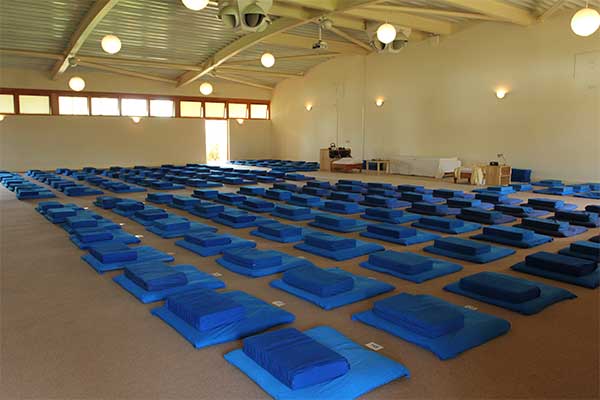
<p>与我共同上课的共有一百二十个人左右，男女各一半。内观楼里大家六十余人分坐在大堂两侧，八行八列。中间是过道，前方摆放着白色的 Dhamma Seat。</p>

<table>
  <thead>
    <tr>
      <th style="text-align: center"><img src="https://yanlin-duan.github.io/assets/pics/vipassana/dhamma_hall.jpeg" alt="内观楼内侧" /></th>
    </tr>
  </thead>
  <tbody>
    <tr>
      <td style="text-align: center"><em>内观楼内侧</em></td>
    </tr>
  </tbody>
</table>

<p>偷偷观察我的同学们是我化解无聊的一个方式。因为不能说话，我仿佛在做一个无声的田野调查。男生这边，大概 50%是白人，30%印巴，5%东亚裔，剩下 15%是黑人和其他族裔。年龄跨度也很大，感觉从二十出头的年轻人到六七十的老爷爷都有。亚裔面孔并不多，算上我只有三人，有一个名字我记成 Takoyaki 的日本小哥，和一个感觉是大湾区最早一代移民的姓 Chan 的老爷爷。还有几位同学给我留下了印象：一个是坐我左侧两个位置之外的梳着马尾辫的壮壮白人，画风让我想起了我的两位前同事 Jordan 和 Eric 的合体。另一个是坐我右前方的朋友，也是个马尾白男，但荧光绿的发色和纹身透露着他的嬉皮属性。哦，还有一个哥们，样子和走路的姿势活像英雄联盟里丧尸布兰德的原画。人真的很有趣，只消一眼，就可以脑补出另一个人的声音、性格甚至故事。我一边钦佩着这种联想和 pattern match 的能力，一边等待着第十天 Noble Silence 结束之后我的种种偏见和脑补一个个被打破的瞬间。</p>

<h1 id="第一日">第一日</h1>

<p>一声锣声把我叫醒。原以为没有闹铃，我可能会起不来（毕竟我是手机闹铃要设八个然后摁掉十次的人）。但其实锣声很响。敲锣的志愿者（我一直以为是课程管理团队会自己来敲锣，但其实是从老生中找了一男一女两位志愿者）会进到我们的楼里，在楼下一声“咣”，在四点钟准时打碎所有美梦。</p>

<p>我虽然没有看到过凌晨四点的洛杉矶，但仅在今年我就已经看过了凌晨四点的苏格兰、英格兰和威尔士。年底之前不如走一趟北爱凑齐凌晨四点英国系列。我边起床穿衣边想。</p>

<table>
  <thead>
    <tr>
      <th style="text-align: center"><img src="https://yanlin-duan.github.io/assets/pics/vipassana/scotland-at-4am.jpeg" alt="凌晨四点的苏格兰" /></th>
    </tr>
  </thead>
  <tbody>
    <tr>
      <td style="text-align: center"><em>凌晨四点的苏格兰</em></td>
    </tr>
  </tbody>
</table>

<p>郊野没有什么光污染。夜空黑的透彻，星星很亮。好像有一颗格外亮的是北极星。我也不确定。勾月挂在内观楼的左前方。我不敢回头看，总觉得回头看会看到另一个月亮。如果真的看到，我或许也不会太过意外。太多魔幻现实的事情已经发生，我可能真的身处 2Q23 年。</p>

<p>天气没有太冷。一件卫衣套抓绒外套就足以保暖。是四点半开始冥想的信号。我快步进入内观楼。锣声又响起。人已经半满。我在门口多拿了两个坐垫，打算今天观呼吸的同时找一找适合久坐的姿势。先试了试盘腿坐 🧘。感觉还可以，但总是不自觉的驼背低头。不够优雅。Goenka 前日说观呼吸时要保持背部挺直，可我又不知道在内观的时候去注意自己的姿势算不算走神，注意到了然后重新挺直又是不是没有做到“觉知而不改变”。不过总的来说，第一天的内观初体验比想象中要好。对于许多人来说的最大难题：走神，我应对的还好。思绪也会飘到不知道哪里去，但通常可以在几秒内意识到，然后重新放回呼吸。不过还是深切地意识到我的脑子，或者人的脑子，就像一个家长盯着做作业的小孩。盯着的时候还好，但一旦放松警惕，就不知道跑到哪里去了：</p>

<p>比如我就在从早上的锣，想到了英文是 Gong，想到了老锣，想到了龚琳娜，想到了龚琳娜和美依礼芽在姐姐第三季里合唱的花海，然后脑中 5 倍速把花海听了一遍。带画面的那种。一切都只发生在我松懈的几秒内，主打一个思路清奇联想离谱。</p>

<h1 id="伙食">伙食</h1>

<p>十天的内观课除了最后一天都只有两顿饭，六点半的早饭和十一点半的午饭。下午五点会有一个小时的茶歇，但只有水果、豆奶和茶。老生只有茶或柠檬水。早饭其实每日都相同：燕麦粥，水果果脯，植物奶（豆奶、椰奶、燕麦奶），水果三件套（香蕉苹果梨），碳水（有麦片、吐司，黑麦面包，米饼）和各式抹料（黄油，花生酱，果酱，还有一些鬼畜的看起来就不是很好吃的酱）。饮料就是茶和咖啡。高中毕业后我就不常吃早餐。连续十天都吃早饭更是很少见的事情。不过口味我觉得无功无过。选择足够多到十天我没有吃腻，也有不错的单品组合（豆奶+巧克力口味麦片+香蕉+吐司黄油+红茶）成为我的无脑选择。碳水很充足。不会觉得饿。只是蛋白质确实比较缺乏。说来好笑，我一个健身又摸鱼了许久的人，“今天的蛋白质吃够了吗”居然是我未来十天可能最担忧的事。倒后来就只能把蛋白质含量最高的豆奶当水喝。感觉中心的豆奶有至少一半是我一个人喝的。</p>

<p>午餐比早餐充满惊喜的多，每一天都不同。但我也不幸在第四天还不是第五天就找到了攻略指南，被剧透了每天吃什么—那就是放在食堂角落的过敏原信息指南。里面详细记录了每天吃什么，原料有什么，甚至还有图。我想到曾经打过的辩题：预知未来是快乐的还是痛苦的。鄙人不才，能预知的唯一未来是之后几日的伙食。对未知的期待消除，对某日午餐枣泥糕甜点的期待出现。正负抵消。</p>

<p>在不能说话的食堂里吃饭，社交准则和男厕所小便池是一样的。大家会先在食堂最远的角落里坐下，之后会相隔一个位置坐。如果是桌子，会先坐对角线。Christopher 每次都是前几个到的，然后就坐到食堂靠窗长条桌最尽头的位置。以至于后来如果我看到别人在他之前坐了那个位置都有些不习惯。午餐有许多绿叶蔬菜，碳水基本靠土豆和面包。除了有几日超常发挥和有几日我觉得蛮不对我口味，基本就是素食版白人饭的水准。</p>

<h1 id="喵呜吧啦啾">喵呜吧啦啾</h1>

<p>早餐+休息时间有一个半小时，绰绰有余。我吃完早饭后又去后花园里走了一圈。在那里我认识了我这十天的第一个好伙伴，一只松鼠。因为一些陈年老梗，我给它起名喵呜吧啦啾。想到这个名字的时候我很兴奋，因为我很确定我是这个世界上唯一一个见过它并叫它喵呜吧啦啾的人。这成了我和喵呜吧啦啾之间的一种特殊的联系。只属于我们的、私密的 bonding。不过喵呜吧啦啾似乎没有我兴奋，它不一会儿就跑去树林深处我看不到的地方了。</p>

<h1 id="集体冥想">集体冥想</h1>

<p>集体冥想一天内共有三次：早上八点到九点，下午两点半到三点半，晚上的六点到七点。因为不能离场的原因，集体冥想对于我来说是很好的判断自己状态的机会—有些时候，比如第一天，第四天，第六天和第九天，我非常专注，在觉知的专注中，对时间流逝的体验很特别。它不像走神一样时间唰的一下就过去了。也不像是过分无聊时寂寞难耐度日如年。它有点像是不需要刻意去数秒也能对过了多久有比较准确的感知。感觉差不多到点了，Goenka 结束时的念诵就会传来。</p>

<p>集体冥想后短暂休息，便是被我称做“留堂”的环节。大家在内观楼重新坐定后，助教便会让部分学生留下，其他人可以回自己房间或在内观楼里继续练习。被留堂的学生们会依次被叫到名字，以 4-5 一个小组的形式去到助教面前。助教会先询问每个人的情况，然后带领小组冥想约十分钟。这也是我第一次除了外貌之外，第一次对同学们有了更多的信息。我知道了我右边的小哥叫 Christopher，左边的小哥是 Carl，长得像我前同事的壮壮白男则是 Sam。</p>

<p>与助教对话的过程就能体会到教学冥想这种“比较玄的东西”的难度。因为去准确描述一种感觉和去检查学生是否做到都是基本不可能的事情。助教问：“能专注地观察自己的呼吸吗？”学生回答：“能。”助教说：“很好，继续保持。”倘若学生说不能，助教则会说：“不要着急，慢慢练习。”我在这些简短的对话里体会到了莫大的孤独感。</p>

<p>这条内观的路，每个人都只能独自前行。没有所谓的感同身受。就算有，这种感同身受也在干瘪的语言输入和输出中压缩失真，信息残留所剩无几。但我又想，这不是根属于冥想的特质，只是因为这件事情纯纯的只发生在一个人的内部而使得它的孤独属性尤为突出。我在创业时也感受过那种孤独，而且最甚的时候不是自己低头做事的时候，而是跟别的 founder 或者跟 advisor 聊天的时候。巨大的信息差使得没有别的 founder 和 advisor 比 founder 自己更了解 founder 正在做的事情。像极了一个人内观自己。所以一切的建议和意见最后都化为“继续保持好的”和“努力停止坏的”。不过什么是好、什么是坏、怎么保持和怎么停止，就是听者自己的功课了。没人可以代劳。</p>

<p>当我听助教和其他学生的对话时，我觉得我像个局外人。于是想到加缪。于是想到他说自杀是唯一严肃的哲学问题。可能伟大的哲学宗教思想都需要一个听起来极端确切、反直觉的、足够小的落点。加缪的落点是自杀。Anapana 的落点是呼吸：倘若没有人可以准确体会我呼吸的感受，那也就没有真正的感同身受。</p>

<h1 id="睡前故事">睡前故事</h1>

<p>下午的集体冥想和留堂都平平无奇。新鲜劲过得很快，第一天还能老老实实照着时间表好好工作的我，到了傍晚时分感觉已经摸清了套路，已经开始琢磨明天怎么摸鱼了。我心态着实超级放松。虽然来之前看了一些博主的文章说内观营怎么怎么苦怎么怎么难，但我倒非常平和，抱持着能做多少做多少的想法。不逼自己抓住每一分每一秒，但求认真时做到最好。很好笑的是，在当晚的“睡前故事”环节（每天七点到八点十五要看 Goenka 的小视频，我称之为睡前故事），Goenka 就说到十天的时间很宝贵，内观成功的秘诀就是持续的练习。我就觉得老哥跨越 30 多年（视频是 1991 年录制的）在这点我呢。事实证明这种被点的感觉会多次出现。这可能就是“要成为宗教/玄学领袖必须有的个人特质”的第二点：足够多的教学经验和洞察人性的能力使得一些话明明是说给所有人听的，但每个人都觉得就是点他自己的。</p>

<p>Goenka 睡前故事的水平发挥不大稳定。我觉得有几日讲的甚好，有几日平平无奇，有几日让人想昏昏欲睡。主题一般有几个：前几日是一些知识普及型的。会讲 Vipassana 的大框架三部分：Sila, Samadhi 和 Panna。简单来说，Sila 就是清规戒律，不偷盗不杀生之类的。Samadhi 是专注力，也就是 Anapana 在训练的。Panna 是智慧，也就是 Vipassana 践行者们所追求的。而这就是通向法（Dhamma）的道路。中期会分享一些励志语录或者寓言故事，我觉得有些还不错，有些确实很有时代感（比如盲人摸象和刻舟求剑），有些则让人直翻白眼（据说古代某某大恶人立志要杀 1000 个人，在杀了 999 个人后遇到了佛，佛教给他内观，他开始内观之后成为了一个大善人的故事）。后期则是我最喜欢的，如何把内观的思想和价值观带到生活中的一些思考和体悟。</p>

<p>将近一个半小时的睡前故事结束，大家稍作休整就开始了新一轮的内观。每天晚上 Goenka 会布置第二天的训练任务。Anapana 的第二天，观呼吸的部位缩小，变成只有鼻腔外侧和上嘴唇的小三角区域。Goenka 说，观察的部位越小，头脑就能更敏锐集中。</p>

<h1 id="一起看松鼠的人">一起看松鼠的人</h1>

<p>第二日。一样的日程安排。我似乎已经习惯了这种朝四晚九的僧侣生活。打坐，吃饭，休息。喝茶。发呆。去树林里走走。我又见到了喵呜吧啦啾。这次，还有另一个同学也驻足观察它。</p>

<p>“一起看松鼠的人。”</p>

<p>这个说法突然出现在我脑海里。我觉得它准确概括了我一半的人际关系。我们在同一条路上走着，偶尔会共同驻足停留，一起看一会儿松鼠。你看你的。我看我的。谁看倦了，就继续往前走。前方或有岔路，我们便分道扬镳；或许没有，我们又会在未来的某个时刻再次巧遇松鼠，然后停下来，站一会儿。</p>

<p>而我和喵呜吧啦啾，则概括了我另一半的人际关系。我注视着喵呜吧啦啾。喵呜吧啦啾做它自己的事。它偶尔与我对视，但我不能强求。我看够了便继续往前走，它并不能强留。</p>

<p>有些时候我是我。有些时候，我是喵呜吧啦啾。</p>

<h1 id="anapana-就像潜水">Anapana 就像潜水</h1>

<p>第三天，继续观呼吸。这次，观察的重点从一呼一吸变成了 sensation（感受）。比如呼出来的空气会比吸进去的空气要热一些。比如气流碰触鼻孔下方的一个小点的时候鼻毛/汗毛微弱的摆动。感觉，就是个很玄妙的东西了。如果说觉察呼吸还是在觉察一个“外界的”东西（气流），觉知感受就开始向内看了。主体从呼吸变成了我。我一开始有点摸不着头脑，因为呼吸本身已经很微弱了，要感受微弱呼吸所带来的温度的变化，所带来的麻、痒、压力或者一些无法被形容的感觉，真的是难上加难。而且有些时候我不信任我的感觉系统，不知道我感受到的是真的还是我想象出来的。就这点我也问了 Kirk。Kirk 说只要不是我刻意在想要某一种感觉，那我感觉到的就是真实的。</p>

<p>我将信将疑，但选择继续实践。Goenka 在睡前故事中也讲到过，如果在这十天对任何理论上的东西无法完全理解和接受，也没有关系。重在实现。可能内观多了，一些理论的东西也自然明了了。我在更大的维度上同意 Goenka 的这个观点。对我，可能也对很多人而言，理论上理解一个东西的难度远低于实践一个东西的难度。有点像所谓的“道理我都懂就是做不到”。我在弹钢琴、创业、滑雪、编程等等方面都有过类似的感受。intellectual 层面的理解和 experience 层面的理解常常有巨大的鸿沟。对于善于或习惯于在 intellectual 层面理解事物的人来说，有些时候会忘记这个鸿沟的存在或巨大程度。这个观点甚至有点阻碍我写这篇文章，因为无论我如何去描述我的体验，都既无法让读者感同身受也无法让读者有 intellectual 层面之外对内观的理解，而实践本身的意义要远大于听我说 Vipassana 教会了我什么。</p>

<p>继续实践下去果真有奇妙的感悟。我发现当我关注呼吸时我的感受的时候，我就仿佛在进行一场精神世界里的潜水。潜水和观呼吸真的有许多相似之处：最直白浅显的，便是呼吸本身的重要性。潜水靠呼吸调节浮力，而内观时呼吸则是此时此刻唯一真实的东西。潜水和内观也都是很个人的互动。极少的与他人的互动。在专注时，整个环境里可以只有你自己。潜水时，你只能看鱼，不能摸它。内观时，你只能看自己的感受，不去改变它。潜水，护目镜一带，满眼望去是蓝色的。内观时，眼睛一闭，主题色是黑色的。当我把这两件事串联在一起，原本无聊和 get 不到的事情也变得有趣和有意义。内观楼成为了一个潜水艇，我们百人一起从艇里游出来，呼吸之间，感受着水流的韵律，等待着不知道什么样的鱼会出现让我们观察。</p>

<h1 id="vipassana-就像洗澡">Vipassana 就像洗澡</h1>

<p>第四天下午，我们正式开始学习 Vipassana。Vipassana 简而言之就是身体扫描，观察全身的 sensation。第一天练习 Vipassana，我们会从头顶开始，几厘米几厘米的向下移动，观整个头皮，脸，脖子，前胸，后背，左右手臂和手，腰臀和两腿。和观呼吸一样的准则：只是觉知，不去反应。在我想到 Anapana 就像潜水之后，Goenka 介绍完 Vipassana，我就觉得 Vipasanna 很像洗大澡。不是那种简单一冲的洗澡。是我实在很脏或者实在很闲的时候把身体的每一块皮肤都搓到的那种洗澡。而且不是不走心地轻轻碰触，是给每一寸肌肤绝对的认真对待。又让我想起了田村卡夫卡在健身之后一丝不苟洗澡的那段描述。</p>

<p>身体扫描对我来说的第一大问题就是看不见。我的身体是空的。就像是有个洞一样。譬如我专注在我的前胸，甚至开始想象我的前胸（按理说不应该有任何画面的具象，应该要把全部精力用于感受），我会什么都感觉不到，仿佛我没有胸。在跟助教的交流后听起来这是很普遍的一个问题，简单来说就是观的还不够多。按照 Vipassana 的理论，身上的每一寸每时每刻都有着 sensation 在发生（甚至身体里也是），所以观不到并不是没有 sensation，而只是 mind 还不够 sharp，或者观察的还不够认真。有一些小的诀窍可以帮助大家找到感觉，比如尝试观察衣服接触皮肤的感觉，但对我来说，即使这个也非常微弱，而且没有接触的部分依旧没有觉知。这个问题在未来六天的内观中有所好转，但直到最后我也依旧有部分位置看不到。相比较而言，我的头皮，脸，腿就很好看。好看到可以指哪儿打哪儿。就像镭射一样，我聚焦到任意一个点上，都可以觉知到那一个点此时此刻的感受。</p>

<p>身体扫描的另一大难点就是打坐不换姿势所带来的疼痛。从第四天起我们开始践行 Adhitthana，在每天的三次一小时集体冥想时尽量不改变姿势。我一开始尝试的半莲花不仅不够优雅，而且会背部酸痛。后来我又开始尝试跪坐：在两腿之间垫三个垫子，两腿叉开跪坐在垫子上。尝试之后发现背会不自觉的挺直，非常舒爽。唯一的问题就是膝盖会痛腿会麻。尝试了两天后我觉得没有完美的冥想姿势，腿腰膝盖总要至少疼一个。也是从这一天开始越来越多人换成了用椅子（男生这边一开始可能只有三四个人，最后有十几个人都坐在椅子上内观了。之后内观室侧面和后面的墙边都摆满了椅子）不过我决定咬牙坚持下，毕竟想体验最原汁原味的内观。而且 Christopher 和 Carl 甚至从一开始就一动不动。我不能输。</p>

<p>在还没有跟疼痛和解的时候，一小时的集体“洗澡”着实有点折磨。前半小时还好，我大概可以扫个三四遍身体，感觉自己干干净净。然后腿就开始痛。一般是膝盖先起反应。先是一个点。然后逐渐扩大。是那种从骨头往外波状扩散的痛。脚因为跪着有些折叠，也会开始发麻，疼痛。因为这些疼痛接下来的十分钟就会开始不专心。明明扫着左臂，可能注意力也会被带去右脚。再十分钟后就基本完全躺平了。偷偷睁眼回头看看还有多久。发现还有二十分钟。度秒如年。看看 Christopher。果然一动不动。内心戏逐渐多了起来。澡反正是不洗了，能姿势不变就是胜利。</p>

<p>到了最后五分钟，无比期待 Goenka 的气泡音的出现。当他真的开始吟唱时，我都开始摇摆，感觉非常悦耳，腿好像也不疼了。再一次感到疼痛就是结束了可以休息想要站起来的时候，大概率是一下子站不起来的，要缓缓起身并按揉膝盖。不过起来之后走一走，抖抖腿，五分钟后疼痛倒也就完全消失了，不会造成什么长期的影响。</p>

<p>最好笑的是我又被 Goenka 跨越三十年预言到了。当晚的睡前故事，他就讲了学生普遍的心路历程—我也普遍了。Goenka 对于为什么会有疼痛又有一套很佛教的解读。他说疼痛是 Saṅkhārā 从身体内部浮现到身体表面的体现。Saṅkhārā 的产生之一就是长年累月对于某些 sensation 的 aversion（厌恶感）。外界人事物会带来 sensation，在内观前人会本能的对 sensation 作出反应（reaction），譬如强烈的渴望（craving），厌恶（aversion）和忽视（ignorance）。而这些正是人痛苦的根源所在。解决痛苦的方式便是停止对 sensation 作出反应，而是观察它。用一视同仁、平静（equanimity）的方式去观察它。</p>

<p>觉知（awareness）和平静（equanimity），就是 Vipassana 的两大核心。我准确地知道此时此刻在我身体的每个角落正在产生的感知，但我以平和的方式去看到所有的感觉，无论是舒适的感受还是疼痛。无论是强烈的感受还是微弱的电流。它们都一样。</p>

<p>都一样什么呢？</p>

<p>都一样无常（Anicca）。</p>

<h1 id="无常">无常</h1>

<p>如果你问我冥想十天学到的最重要的东西是什么，我想大概是无常。不是那种说说而已的世事无常。是从经验和体验层面深刻感受到的普适性的无常。这十天以前我所理解的无常，出发点更多的是我的能力边界。我所能控制的事情之外的所有，是无常的。这里的无常，也并非专注于它非永久或者变化的特点，而是失控和无法理解。内观让我把这个思路推向到了一个极端：我本身就是无常的。</p>

<p>这句话也很容易坍缩成一个明显的事实：人终有一死。这确实没错，但无常不仅发生在一生的宏观尺度，也发生在每时每刻。抽象一点说，人通过一套感受系统来输入外界给他的信息，潜意识和意识会进行反应，反应的结果又会通过同一套感受系统来进行输出。这里的关键就是人对于人事物的反应，其实是会影响感受的。就比如生气的时候可能会感觉头皮在跳，伤心的时候会觉得心脏在痛一样，任何大大小小的情绪都来源于 sensation，也会改变 sensation。然而 sensation 本身就是从微观尺度上一直在变、无法控制的东西。任何感受都是无常的。而人太过习惯对于无常的东西作出反应。甚至当感受本身已经逝去，反应所带来的新一轮的感受、新一轮的反应却还在持续。而在这一轮轮对无常的感受作出反应的过程中，人积累的就是 Saṅkhārā，也是痛苦的来源。</p>

<p>如此，就和 Vipassana 的理论连在了一起。练习 Vipassana 让人不再对无常的感受作出反应，而是平静的观察。在不断的平静观察过后，没有了新的 Saṅkhārā 的出现，旧的 Saṅkhārā 不断浮到表面然后被观察，消失，人就可以断绝痛苦。</p>

<p>乍一听有些玄妙又有些道理。</p>

<p>我对于根除痛苦并没有太大兴趣。现在没有削发为尼的想法。但能少一些内耗，看得明白和通透些，是我想要的人生观和价值观。从这个角度看，内观，观一分有观一分的欢喜。即使我不信这一套 Saṅkhārā 的理论，体悟到我的无常，并且把我的无常前置于世事无常，也足以让我重新思考我与自己，我与人事物的关系。</p>

<p>我在最近的几年逐渐意识到自己自我人格的不完善。说白了就是没有摆正我自己的位置。我对于我的位置。我在其他人那里的位置。我自己和自己在做的事情的关系。我并不是情绪容易失控的人，但许多时候那只是因为我有意无意的忽视或者轻视那些会让我敏感的点。我表面的稳定独立是建立在我把我自己包裹在一个泡泡里的前提下。但有些时候，泡泡会被戳破。有些时候，我都不知道泡泡已经破了而我在往外流。</p>

<p>四月，我们创业公司在融资。那时候觉得有一万件事需要我的注意力。要平衡生活工作、朋友社交和生活独处，感觉 everyone wants a little piece of me。我只觉得累，但没有觉得特别累。直到某日坐在地铁上，我就开始掉眼泪。掉眼泪不是哭，我没有情绪的感觉，首先冒出来的感觉是“哇为什么我突然开始流眼泪，好神奇”。然后是“车厢里别的人看我流眼泪会不会觉得很奇怪”。但我确实那一个瞬间感觉不到难受。流眼泪就像流鼻涕一样。不是被某个情绪戳中了，就是满了溢出来了。停不下来。</p>

<p>后面又有一日，从一大早等某家风投下午给我们打的 decision call。有些悲观，觉得还要约个电话不直接发 term sheet 估计是凉凉了。但又想，之前的许多 signal 还比较正面，而且要拒的话发个邮件就好了，没必要约个电话。然后就开始干呕，恶心想吐。第一反应是：“你又怎么了。等高考成绩都没有这么大反应，一通电话至于吗？”第二反应是：“记得在知乎还不是哪儿看到说人的任何情绪到了极端都是想吐。”</p>

<p>在我身体扫描时我想到了这两个瞬间。有些后怕。我的身体一定当时已经有各式各样的感受了可是我看不到或选择不去看。最后生理上的反应比情绪上的反应来的还要早。</p>

<p>我过去知道泡泡会破，所以我会找一个刺少的地方放置我的泡泡。熟悉的环境。擅长的事。爱我的人们。建好模型可以理解的世界。可我后来发现，环境我无法控制，事我无法控制，人我无法控制，这个世界我更 tmd 无法控制。</p>

<p>但这些都不是泡泡会破的原因。这些外界的因素本身都不带刺。是我对他们的执念，对他们的期待，对他们的渴望，厌恶…种种反应将它们从一个个温润的点变成尖尖的刺，指向我自己。</p>

<p>这场人生的游戏里，只有我是我自己的破壁者。让我的人格不完整、不稳定的，只有我自己。是我允许我自己被伤害。但无常的一切本没有伤害，是我对它的幻想、反应从内部攻击我自己。</p>

<p>Vipassana 的意思是“如实观察如其本然的实相”。英文就是 to see things as is, not as you would like it to be。事情本然的实相，便是无常。</p>

<p>我深以为然。</p>

<h1 id="三只松鼠">三只松鼠</h1>

<p>第五日午休的时候去后庭走，同时看到了两只松鼠。次日，又看到了一只身型明显更小的松鼠。由此我得出一个令人有些伤感的结论：这片树林里至少有三只松鼠。</p>

<p>之所以令人有些伤感，是因为我并无法判断那两只身型较大的松鼠有什么分别。这也就意味着，我前几日跟同学一起看到的那只，可能不是喵呜吧啦啾。这两只也可能都不是喵呜吧啦啾。</p>

<p>我以为的我与喵呜吧啦啾的联结，那种全世界只有我有的联结，在它消失在我的视野的那一刻就消失了。我没有足够的信息去识别它，更别说找到它。即使我能识别它，能找到它，喵呜吧啦啾可能也不是当时的那个喵呜吧啦啾了。就像此时此刻的我，在意识到无常之后，也不再是之前的我了。我们都像忒修斯之船一样，不断变化。那我们的关系又怎么可能是永恒的呢。</p>

<p>脑海中又开始播歌。今天点播的第一首是罗大佑老师的《恋曲 1980》。</p>

<p>“你曾经对我说，你永远爱着我，爱情这东西我明白，可永远是什么。”</p>

<p>第二首是小众歌手孙燕姿的《开始懂了》。</p>

<p>“原来人会变得温柔，是透彻得懂了，爱情是流动的，不由人的，何必激动着要理由。”</p>

<p>第三首是李宗盛大哥的《当爱已成往事》。</p>

<p>“不要问我是否再相逢，不要管我是否言不由衷。为何你不懂，只要有爱就有痛。”</p>

<p>我的妈耶。不吃几本经书打几年坐这些神仙是怎么写得出唱得出这些东西的。</p>

<p>流行音乐喜欢以爱情为题眼。不过说一句俗的不能再俗的话：他们说的不是爱情，说的是人生。</p>

<p>不论我与喵呜吧啦啾是否已见过，是否会再见，都希望我们各自安好吧。</p>

<h1 id="接连下雨的几天">接连下雨的几天</h1>

<p>第六日开始下雨。一开始只是晚上下雨。早上起来后望向内观楼和天空，想象着那画面是类似红楼梦的古装电视连续剧的片头。右下角用行书写着“第六日 空山新雨后”。</p>

<p>那之后几日，每天都有一句诗词。</p>

<p>第七日天气阴沉一整天，是为“第七日 暮霭沉沉楚天阔”。</p>

<p>第八日，风极大，我题作“第八日 树欲静而风不止”。</p>

<p>感觉身体里沉睡的文化修养又开始复苏。许多背过的古诗词并不是就没了，他们只是需要一个锚点从记忆体的深处被唤醒。</p>

<p>天气不好，人也开始倦怠。我有两日早上起不来，想摸鱼睡过 4:30-6:30 的冥想，直接听着 6:30 的锣声起床去吃早饭。结果听到锣声起来，发现天色亮的不可思议，大家也并不是往饭堂的方向走，而是匆匆走进内观楼。原来我不仅睡过了冥想，甚至错过了早饭！心中大喊不妙，错过了一整天 50%的饭，虽然打坐不消耗什么卡路里但还是会担心肚饿。</p>

<p>大风之中的树林又有不同的风景。我先是注意到了树干上的刻痕。明明这些刻痕一直都在我却在第八日才看到它们。可能是因为我前几日就注意到有一块立牌写着不要在树上刻字，我便假设了来这里的都是文明人，不会有人在树上刻字。</p>

<p>但树上的字确实也很有意思。有一处写的是 WE ARE ONE，我觉得是谁悟了，在树中看到了自己，或在自己身上看到了树，于是激动地刻下。另一处就更朋克了，刻了个 PLEASE DO NOT LEAVE MARKS ON THE TREE.</p>

<p>离谱，真的离谱。</p>

<h1 id="第八天的躺平和意外">第八天的躺平和意外</h1>

<p>第八天可能是我最难的一天。完全无法专心。只想睡觉和摸鱼。反复思考为什么今天是第八天今天是第九天就好了，明天就是最后一天了。</p>

<p>有意识的摆烂。第四天学习 Vipassana 之后，我们每日就在练习不同的“洗澡技法”。最一开始是从头到脚洗。然后是从脚到头洗，然后是对称着洗（同时观身体的两侧），然后是泡澡（同时观整个身体）。集体冥想的时候我澡也不洗了。早上开始空气弹琴。海顿奏鸣曲里左手的阿尔贝蒂低音弹得很不均匀，我就开始一点点从慢到快的练习。练了一个小时空气琴，感到满足。下午更无聊，决定精进英雄联盟打野技术。我开始量子训练。把能想到的野区英雄的第一轮刷野都过了一遍。又开始思考怎么抓人。脑中模拟各种极限操作 1v9，上演了一万场精彩的五杀。当然，作为一个合理的模拟器，也要思考劣势局和失误。开始复盘最近几局跟烨哥的双排，我哪里可以处理的更好。集体冥想结束后，我激动不已，再次希望今天是第九天这样明天结束了就可以回家打游戏带烨哥上大师了。</p>

<p>游戏和音乐确实是我排解无聊的主要方法。弹琴累了就听听歌。听歌无聊了就打打量子游戏。偶尔想要再努努力的时候就会把 BGM 改成巴赫。巴赫三部创意曲之五（降 E 大调）真好听啊，不会太浪漫，又不会太激昂。平和的旋律。适合冥想。equanimity。</p>

<p>就是太短了，播一遍也就三分钟。澡速速洗完，又开始打野。</p>

<p>只可惜英雄联盟也玩不了多久。倒不是游戏的错，主要是因为当天的午饭有许多豆子。我起初还很高兴，感觉植物蛋白也是蛋白，多吃大豆就不用吨吨吨豆奶了。但奶足豆饱之后才发现好像事情并不简单。整个下午在内观室里，游戏每想几分钟，注意力就要转移去控制另一些事情。然而很多事情都是在我的控制范围之外的。即使能够控制，我也只能控制一部分。比如声音。控制声音也有一个问题。老话说的好，xxxx，xxxx。安静的往往更有威慑力。我又只得用冥想毯把自己包裹住。又担心侧漏，用冥想垫挡住，超级加倍。空气分子也是无常的。随时随地都在运动。我可以减缓渗透的速度但耐不住我吃的是真的多。只能开始用力呼吸，试图回收。同时眯缝着眼睛看身边人有没有表情的变化或者一些厌恶的动作。</p>

<p>我看向 Christopher，Christopher 一动不动。</p>

<p>我看向 Carl，Carl 突然一声冷笑。</p>

<p>一定是因为他内观有了令人欢喜的收获。与我无关。</p>

<p>希望身边人扫描身体的时候不要太专注于鼻子的感受。阿弥陀佛。</p>

<p>可能唯一给我慰藉的，就是内观楼里不时会有此起彼伏的异响，让我知道我不是在孤军奋战。</p>

<p>第八天晚洗了个真的大澡。假装无事发生。</p>

<h1 id="第九天">第九天</h1>

<p>第八天晚的睡前故事，Goenka 说，明天第九天将是你们最后一天认真练习的一天。因为第十天，Noble Silence（神圣的静默）将被解除，大家可以说话。也因此，那日会有许多干扰，练习将不再能如静默时那般专注。我还是想做个善始善终的人。中期鱼也摸了，最后静默的一日就尽力去做吧。</p>

<p>其实我还挺喜欢 NS 的。喜欢那种可以理所应当目中无人的感觉。本来跟陌生人对视就有些尴尬，现在可以正大光明的移走视线或者干脆看地，即使面对面走来也可以不必（不能）点头示意 say hi，很爽。我再次确信自己骨子里是个 I 人。又想到自己上学时候很喜欢上课接下茬。人是会变的。Anicca，Anicca，Anicca。</p>

<p>但我也想好了明天要去聊的人。上述我仔细观察过的同学我都还挺想聊一聊，看看我猜的有多离谱的。但又有些社恐不知道要怎么开场。“Hey！我关注你很久了，要聊聊吗？”听起来有些变态。最好他们来主动找我搭话。或者在我和其他人聊天时自然加入。但自然加入这件事情我就不大会。有点难判断什么时候一个人说完了，还是只是换口气继续输出。曾经有过那种我想了一句非常应景的回应可对方一直 blablabla 到我的梗都接不上了才停，也有那种我暴力插入结果同时跟别人说话显得我很没有礼貌的尴尬场景。哦，还要自我介绍一百遍。如果有新的人加入又要介绍一遍。我融资的时候已经介绍麻了。我累了。</p>

<p>跟不熟的人在没有共友、没有其他活动的纯社交环境 social，太难了。</p>

<p>第九天确实颇为专注。也收获颇丰。跟疼痛的成功和解是一个里程碑。其实正如 Goenka 说的，疼痛的很大一部分是心理作用。心理上你觉得不舒服，想逃避，就会越来越痛。如果只是平和的、客观的、准确地观察它，是具体哪里痛，怎样的痛，其实过一会儿它就会消失了。痛，也是无常的。</p>

<p>我确实有此体会。我之所以在上文可以准确的描述我腿的痛感，就是因为我仔仔细细地观察过了。哪里是钻着疼，哪里是酸痛，哪里是隐痛。同时不能给腿多过身体其他部位的注意力—这也很重要。腿的疼痛和衣服扫过后背的感受和头皮的电流感都是一样的。确实不一会儿，疼痛的感受就消解了。不是不痛，或者麻木了，而是感受消解了。有点像发烧的小孩子虽然还烧着，但不再哭闹了。</p>

<p>另一个里程碑是心态上接受看不到的事实。在努力了几天之后前胸后背的一些位置依旧是空白的，没有感知。我第八天晚上洗大澡的时候特地把自己摸了一遍，想记住这种触感，可依旧没用。Goenka 说如果感受不到 sensation，就停留一分钟，停留一分钟依旧感受不到就移动到下一个区域，没有关系的。接受现在的状态就是感受不到。See things as is, not as you would like them to be. 不要产生厌烦焦虑或者难过的心情。有这些反应也会产生 Saṅkhārā，就失去了我们内观的意义。我觉得这可能是最底层的与自己的和解。和解首先需要有能觉知现实的能力。其次要有能够接受现实的心态。最后要有能够承认自己能力不足的勇气并平和的面对它。我觉得当我可以接受我就是看不到我的一些部位时，我好像更爱我自己了。在内观的修行上，人与人的攀比本就没有意义。那我骗我自己或不能去接受这是一个需要时间和努力的过程就更没有意义。就像从经验层面上接受了无常一样，我也从（内观的角度上）更底层与自己和解了。</p>

<p>我在森林的边缘看到了一只兔子的尸体。头已经烂开，有蝇在上面飞。在内观中心看到死去的生灵是一件蛮少见的事。我不知道发生了什么。希望它没有痛苦。</p>

<p>第九天的睡前故事是我最喜欢的。Goenka 分享了要如何在生活中践行在内观中领悟到的这些道理。诸如无常。诸如如实观察事物本真的样貌。诸如平和。他做了一个比喻，说有一个画家画了一个大美女，然后疯狂的迷恋上了她，众人都觉得他疯了，爱上一幅画；又一日，他画了一个恶魔，然后害怕到夜不能寐，众人觉得他更疯了，厌恶一幅画。可我们每个人又何尝不是一个画家，我们所看到的每一个他人，都不过是对方在我们心中投影的一幅画罢了。我们爱的恨的，去作出反应的，与那个画家无异，都只是对着一幅画罢了。</p>

<p>他又说，我们对一个人的了解是如此的少，可能许多年前，某个人对你做恶，你一直记在心里，多年之后相见，只是看到这个人的脸，身体自然就会有反应觉得对方是个坏人；然而这么多年可能这个人早已变了我们却不知道。的确，我们对一个事物的判断，无论是从时间还是空间的任何维度来看，都是如此片面。事物本又无常。在这么多变化中，哪里来的那么多大爱大恨呢。</p>

<h1 id="第十天">第十天</h1>

<p>随着早上的集体冥想结束，走出内观堂，Noble Silence 也结束了，正式开始了 NS（Noble Speaking，神圣的对话）。</p>

<p>最先开始的是眼神交流。大家的视线不再避让，四目相接会点头微笑示意。我还是社恐，不知道该在哪儿呆着，跟谁说话，自己先小声哼哼了几声，感觉自己的声音和印象中的声音不大一样。太久不说话好像声带还不习惯震动。
我一头扎进了树林里。没走几步路就看到了 Carl 和 Sam 在聊天。他们看到我也跟我打招呼，我的出关第一句话很可惜不是 hello world 而是 hey what’s up guys。</p>

<p>我还在想他们怎么这么快就熟络起来，聊起天才发现，Carl 和 Sam 本来就认识，相约一起来内观营。Carl 说他们是高中同学。我还有些意外，因为 Carl 很明显的美式口音，Sam 则是英国腔。原来他们之前都在迪拜读高中，后来 Carl 回了加拿大，现在又来了英国，住在 Sam 附近的城市（利物浦附近）。</p>

<p>我们三人一起在树林里走了几圈，又在草地边的长椅坐下。我们从过去九天的冥想体验聊起，什么时候觉得通了，什么时候又觉得最难熬。哪天最想破戒，有没有想要离开的冲动。Sam 说他第四天感觉已经是极限了，非常想逃跑，可是是 Carl 开车带他来的，他还得先从 Carl 那里把车钥匙偷到，感觉太过麻烦只得就此作罢。我们都哈哈大笑。我问他们如果认识彼此又不能说话这几天会不会很难熬，Carl 说他感觉还好，毕竟在内观室并不挨着（中间隔一个人），回到房间大家都有帘子隔着，不刻意地话其实可以一天都不跟对方接触。（我真的完全没有看出来他们认识，比如吃饭的时候也没有印象他们总是坐在一起或者会对视/窃窃私语）。</p>

<p>Carl 和 Sam 感觉是两个 E 人。Sam 我并不意外，举手投足中真的都和我的前同事 Jordan 很像。Carl 比我想象中也健谈许多，高冷学霸光环破灭了。</p>

<p>另一位学霸 Christopher 的光环也小小破灭。我本以为他会是六根清净的人设。第九天看到他约了跟老师的 1 对 1，我都在想是不是他在问如果想要全职修行、剃发为僧的步骤是怎样的。结果 Christopher 是个甜甜恋爱人设。他是跟他女朋友来的，一个印度裔的小姐姐。他俩自从 Noble Silence 解除可以在规定的区域内男女聊天，就一直黏在一起对话。也没看 Christopher 跟别人说话，我也不好意思去当电灯泡跟我的邻居 say hi。</p>

<p>午饭时 Takoyaki 坐到我旁边，我们也聊了天。我先是夸了他很认真，说我有几天早晨四点半到内观房时发现他已经在了，后来累了想回房休息一下再继续，他还一动不动地披着毯子在那里打坐。他用非常日本人地谦虚感回复我说他觉得自己冥想的很差，一点都不认真。原来 T 桑十几年前就在东京上过一次十天的内观课了，多年之后再来英国，感觉之前学的都忘得差不多了。我问他是什么让他想要再来一次内观营。他说他最近被谢菲尔德大学的哲学博士项目录取了，入学前正好有一些时间。他本身也是对于 morality 和 mind 很感兴趣，觉得在哲学的理论学习之外，冥想也是一种实践。他还跟我分享了关于开小差的科学/哲学理解，为什么人会 mind wondering，mind wondering 的不同阶段等等，挺有意思。</p>

<p>后面还有好几个人主动来找我搭话。原来不仅我在偷偷观察别人。很多人也在偷偷观察我。有一个叫 Vivek 印度小哥看到了我有一日穿着我前司的衣服，最后一日特别来找我聊几句，他在 London 的 Meta 做 engineer manager，也是之前从湾区到了纽约又到了伦敦。人听上去很厉害，之前也是搞竞赛然后肉身翻墙直接在印度被招到 Facebook MPK。我本来想秀一下我的人脉，结果耐不住 Meta 实在太大，似乎没有共友。只得相约次日能用手机之后加一下好友，靠社交网络帮我挽尊。</p>

<p>坐我左前方经常摸鱼的小哥也凑过来跟我打招呼，但他的印度口音有些重我实在没有记住他的名字。他说他是先看到了内观室外面有一个我在的创业孵化器的水壶，就想知道是谁的，最后观察到了我。原来他也是个 founder，他们是做 climate tech 的，大概就是用数据库和算法来计算消费者消费的碳排放的。我一听就知道我们一定可以从 B2C 到 B2B2C 的艰难旅程中 bonding 一下。果不其然他们一开始也是天真的觉得可以直接 2C，然后被市场爆锤后开始找寻跟银行合作的机会。当然，作为初创企业把产品卖给银行也是一件令人头大的事情，漫长的销售周期，不清晰的 decision maker 和 budget holder，大企业的官僚主义…样样都是可以杀死一个公司的毒药。关键是这毒药并不是立即发作的，是一个慢性毒药，中间还会多次给你是解药的希望。就在这情绪的过山车中，小哥也有些 burnt out，感觉经常被愤怒和焦虑缠身，于是来到山中内观，找寻一下内心的平静。</p>

<p>我还认识了 Ed，是摸鱼小哥的室友。Ed 是一个 film location scout，我之前听都没听过的职业。他做的事就是帮电影导演选电影拍摄地，然后拍摄样张，再 pitch 给导演团队。如果选中了就会负责当地的联络事宜：拿到拍摄许可，安排整个团队的车停在哪里，如果没有网络要提前过去把网络设置好，如果需要还得联系政府设好路障，等等等等。听他讲他的工作，感觉就是一个有超多体力活+沟通需求的开放世界解谜游戏：毕竟电影+场地的不同就会使得每一个项目都有着独特的挑战，很难套公式。Ed 也不是科班出身，本身读国际关系的他，因缘际遇走上这条路之前，也去非洲当过 builder，欧洲当过英语老师，在学校做过 RA，在伦敦当过公务员，但最后公务员的官僚作风让他觉得作为一个纳税人他的钱就被扔进一个如此低效地系统实在令人痛心疾首，于是半年后就果断裸辞，然后拥抱对电影和旅游的喜欢，走上了 location scout 的路。听他讲这种项目制的生活状态（如果想闲一点可以一年只工作半年，想忙一点可以项目不停轮轴转），讲跟各种有名的导演和演员打交道（他帮魔戒选了址！）谁很 nice 谁耍大牌，还有看到自己名字出现在电影结尾 credit 的名单上时的感受，感觉对我来说就是另一个世界。我最后一天还在愁怎么回伦敦，因为星期日早上七点闭营而星期日第一班公交车要到十一点才有。我随口问了句 Ed 他怎么来的，Ed 说他开车来的，然后问我需不需要搭他车回去。当时又感觉到世界上有许多爱和善意，我和 Ed 萍水相逢，第十天聊天前我甚至没有注意到他。后来我跟 Ed 相约他年底从巴西玩回来后伦敦相见，请他喝酒 🍺 :)</p>

<p>下午在食堂外的空地上，大家继续围成一个圈聊天。course manager Patrick 和 Will 也加入我们聊天。一开始我以为 course manager 都很高冷，要维持管理者的那种严肃气质。但后来发现他们也就是 server（志愿者服务人员）团队里的一员，和厨房里做饭的 server 没有差别。我问 Will 那为什么你会是 course manager，他说他也不知道为什么，这是他第二次做 server，上一次做完这边的总负责人就说 Will 你下一次再来去试试做 course manager 吧，正巧 Patrick 是一个比较有经验的 course manager，于是就让他们俩搭伙。我问 Will 你上一次做 server 是什么职务，他一笑说我是主厨！我很诧异，问他说你是不是很会做饭，所以申请的时候他们就把你放在了主厨的位置上，他说完全不是，他一点都不会做饭，不过没有关系，这个冥想营的运动机制就是规范化流程，所有人都按照列表办事，怎么洗蔬菜怎么切菜怎么做饭全都有傻瓜指引，这就是这么多年办营留下来的经验总结。“就连 course manager 也是一样的”，Patrick 说，并从他和 Will 都随身带着的小挎包里拿出一张纸，上面写着几点要在哪儿做什么。原来这就是依靠（可能毫无经验的）志愿者也能有效运作的秘密！</p>

<p>大家也聊起了这几日的见闻和趣事。第一个话题便是兔子的尸体。有一个在苏格兰开酒吧的大哥说他觉得这兔子是被 polka（猎鹰）猎食的。这就是为什么它的头已经不在了。另一个哥们接了一句说最近森林里好像确实有专门猎食兔子的生物，几日前他在宿舍区边上看到了另一只死兔子，无独有偶绝非巧合。</p>

<p>死亡或许太过沉重，于是又聊到饮食。豆子宴是绕不开的话题，大家听到 beans 就会心一笑，知道这话题的走向是什么。不过一个印度大哥经历清奇，他说豆子对他有别样的效果。那天刮大风又有点飘雨，外面阴冷，但食物却暖心又暖胃。他水足饭饱之后，从温暖的食堂，穿越阴冷的户外走到温暖内观房，坐定准备下一场的集体冥想。他觉得冷风吹过又到了温暖的室内，裹着毯子，脸颊热热的，呼吸平和且温柔。他开始内观，好像看到了许多粉红泡泡。</p>

<p>他记得的下一件事情就是他打了个呼噜，头一坠，醒了过来。</p>

<p>Carl 噗嗤一声笑了，说我听到你打呼噜了，那天都把我逗乐了。</p>

<p>我也噗嗤一声笑了，心想原来 Carl 那天笑是这个原因。</p>

<p>我也非常佩服老哥，讲起自己的糗事一点都不尴尬。可能出糗也无常吧。</p>

<p>最后一个大家常聊起的话题就是之后还会不会再来“复读”，以老生的身份再来冥想营。</p>

<p>我说我觉得对我来说，这十天的冥想课就像搬家前的整理和大扫除。我仔细梳理一遍房子里的东西，把可以扔掉的扔掉，把想要带走的留下。我不知道什么时候我会搬下一次家，有可能是人生到了一个新的阶段，或者是对现在生活的环境感到不满想要调整和改变，又或者只是机缘巧合。我虽然不知道什么时候会搬家，但我知道我不会一辈子不搬家。当那个时刻到来了，我就需要一次大扫除了，我就会回来了。</p>

<p>下一次，我想去尼泊尔那边的中心，据说从最近的城镇要开吉普四个小时才能到达。每天一睁眼，便能望见喜马拉雅山的日出。</p>

<table>
  <thead>
    <tr>
      <th style="text-align: center"><img src="https://yanlin-duan.github.io/assets/pics/vipassana/dhamma-shringa.jpeg" alt="尼泊尔喜马拉雅山脚下的内观中心" /></th>
    </tr>
  </thead>
  <tbody>
    <tr>
      <td style="text-align: center"><em>尼泊尔喜马拉雅山脚下的内观中心</em></td>
    </tr>
  </tbody>
</table>

<h1 id="结语">结语</h1>

<p>在我消失的那十天里，世界依旧运转着。我和同学们第十日还在说世界上肯定有大事发生了，只是我们都不知道。当时的三大候选新闻就是台海开始了、拜登挂了和俄乌结束了。次日允许用手机后，我打开 CNN，看到满屏的巴以战争。三大头条候选新闻都没有发生，但发生的并没有更好。那是一种颇为割裂的感受：一百余人在山里好吃好喝，冥想打坐，用梵语念诵着希望众生快乐。六千公里之外，炮弹横飞，尸横遍野，两个源起一家的种族因为不同的宗教信仰矛盾愈演愈烈直至横刀相向。</p>

<p>这篇文章的许多内容我早就在内观营摸鱼休息的时间构思过。本来以为出营后两天便能奋笔疾书的写完，最后因为种种原因花了一个多月才写罢。飞机上依旧是码字高产地。我在去奥地利的飞机上写、回英国的飞机上写、回北京的飞机还在写。写的我都用出了几个苹果备忘录软件的 bug。不知道是不是文章太长，还是中英文混杂，光标经常乱跳，本来是写在备忘录最末的段落突然就被插到了中间某处，只能返回重新打开备忘录，然后狂摇手机撤回。同时眼光扫射身边人会不会觉得我是用微信摇一摇的那种人。在此要特别感谢身边催稿的小伙伴，是你们的期待让这篇我给我自己一个交代的意识流万字长文得见天日。</p>

<p>这篇文章的唯一一个目标读者就是我自己。主要是写此文的此时此刻的我自己。次要的是未来的某时某刻的我自己。一个月已经是足够的时间让我体会到这篇文章的前半段本是刚刚发生的事情，但感受已经慢慢褪去，记忆已经慢慢模糊。以至于写文章的后半段的时候，我担心许多文字已经失去了第一人称的温润触感，而转向了第三人称更冷静更客体更有事说事的视角。我不想写违心的话，于是更难落笔。然而拖延的每一天都不会让那种第一人称的感受更容易回来。只能专心地回忆并观察自己试图找寻一些蛛丝马迹。于是再次感受到无常。人的冲动和热爱也是无常的。如果难得的对什么人对什么事有了奔头就去做吧。不过在行动的同时要放平心态，不然就会忘记享受过程而期待结果，并在期待产生落差的时候感受到痛苦。</p>

<p>No craving. No aversion. No ignorance. Maintain perfect equanimity.</p>

<table>
  <thead>
    <tr>
      <th style="text-align: center"><img src="https://yanlin-duan.github.io/assets/pics/vipassana/dhamma_hall_2.jpg" alt="走之前拍摄的内观楼" /></th>
    </tr>
  </thead>
  <tbody>
    <tr>
      <td style="text-align: center"><em>走之前拍摄的内观楼</em></td>
    </tr>
  </tbody>
</table>]]></content><author><name>Alan Duan</name><email>duanyanl97@gmail.com</email></author><category term="Life" /><category term="Life" /><category term="Meditation" /><category term="Vipassana" /><summary type="html"><![CDATA[]]></summary></entry><entry><title type="html">北美乔迁伦敦安家指南</title><link href="https://yanlin-duan.github.io/life/settle-down-in-london/" rel="alternate" type="text/html" title="北美乔迁伦敦安家指南" /><published>2022-06-20T00:00:00+00:00</published><updated>2022-06-20T00:00:00+00:00</updated><id>https://yanlin-duan.github.io/life/settle-down-in-london</id><content type="html" xml:base="https://yanlin-duan.github.io/life/settle-down-in-london/"><![CDATA[<p>这篇文章本来想写在公司的Wiki里的，但一直拖延就没有了机会。于是决定直接用中文写个短的，发在博客上。</p>

<h1 id="context-and-disclaimer">Context and disclaimer</h1>
<p>本文针对的读者是从北美因各种原因需要乔迁来伦敦一段时间的科技公司的朋友们。其中很多内容可能也并非北美-specific / 科技公司-specific，读者可以自行斟酌拿捏。</p>

<h1 id="最重要的几件事">最重要的几件事</h1>
<p>这几件事是如果不做之后可能会比较麻烦的，所以先列出来：</p>
<ol>
  <li>
    <p>检查常用App是否绑定了手机号2FA并解绑</p>

    <p>如果你的美国手机号不支持国际漫游或者你不打算打开国际漫游并有一个备用手机（主手机不是双卡双待的）来接收短信验证码的话，就需要提前先解绑自己的美国手机，然后可以换成一个google voice的手机号，或者就等来了英国用英国手机号重新绑定。</p>

    <p>比较重要的需要检查的app有：</p>
    <ul>
      <li>银行账户</li>
      <li>炒股软件</li>
      <li>公司发RSU的平台 / 401K的平台 / Benefits / Health insurance的平台（需要的原因是美国的报税期你可能在英国，可能需要登陆下载tax document）</li>
      <li>信用卡</li>
      <li>社交软件（Facebook, Telegram, WeChat, WhatsApp etc.）</li>
      <li>过一遍自己手机里常用的App和浏览器bookmark的网站，看看有没有漏网之鱼</li>
    </ul>
  </li>
  <li>
    <p>取消没必要的信用卡/服务订阅</p>

    <p>有一些信用卡的offer和perk是只有美国能用的（比如Amex Plat的Uber credit），如果没有好的用法或者美国的消费可以取消。</p>

    <p>服务订阅的话，YouTube, Netflix, Apple Music, Spotify, Disney Plus这些英国都可以正常用，Hulu, YouTube TV, Peacock, ESPN, HBO Max都是英国用不了的（有些用VPN也没有办法）。Amazon Prime和Audible英美也是不通的，建议取消美国的，看情况定英国的。（但Audible有一个办法继续使用美国的credit在英国买书，简单来说就是用VPN/想办法到美国的Audible网站上选择gift this book，然后再用自己的任何账号redeem就可以了）</p>

    <p>Lyft英国是没有的，一般都用Uber和Bolt。但伦敦公共交通足够发达很少需要打车。</p>

    <p>Doordash英国也是没有的，这边一般用<a href="https://roo.it/aland-1f9w">Deliveroo</a>，Uber Eats或者<a href="https://apps.apple.com/us/app/hungrypanda-food-delivery/id1119397292">HungryPanda</a>。</p>
  </li>
  <li>
    <p>更改自己的地址</p>

    <p>最重要的地址应该是银行和公司内部系统吧。如果有英国的地址且可以改成英国地址的话，可以改。否则的话可以改到朋友家，然后写care of:</p>

    <p><em>你的名字</em></p>

    <p><em>c/o 朋友的名字</em></p>

    <p><em>朋友家的地址</em></p>

    <p><em>XY, 12345</em></p>

    <p><em>United States</em></p>
  </li>
  <li>
    <p>驾照续命</p>

    <p>在英国的第一年可以使用美国驾照。所以如果美国驾照快过期了，在英国又觉得会在英国/欧洲租车出去玩的话，可以想办法提前续一下驾照的到期时间（当然如果是H1B未中的小伙伴，可能因为OPT的限制也没有办法延长了……）</p>

    <p>也可以研究下办一个<a href="https://www.aaa.com/vacation/idpf.html">国际驾照</a>。我简单搜索了一下如果用美国驾照办国际驾照一定要在美国办。不过我本人并没有办过，所以没有更多这方面的经验分享。</p>
  </li>
  <li>
    <p>提前申请申根签证</p>

    <p>如果打算去欧洲玩又需要申根签证的话，可以在美国的时候就先提交了在伦敦的<a href="https://fr.tlscontact.com/gb/lon/index.php">申根签证</a>的申请。申请最多的应该是法签。今年据说提交材料已经要三个月后了，所以赶紧先注册填表交钱把时间约上比较好。</p>

    <p>法签前两次一般比较抠门，第一次去几天给几天，第二次一般给到半年，第三次及以后可能可以开出一年签或多年签。具体攻略小红书上有很多。</p>
  </li>
  <li>
    <p>洗牙与拿药</p>

    <p>美国牙科保险一般都会包一年两次洗牙。英国NHS（全民医保）不包，如果走NHS洗牙一般要排好几个月的队，然后要自费20多镑。私立全部自费的话可能要小100镑。所以能在美国搞定最好。</p>

    <p>开药则相反。英国这边一些常见的处方药都是一个价（£9.35），而且拿药体验极好，不用各种打电话催保险催药房用coupon，Boots（即英国的CVS）街上很多很方便就能取到药。所以如果有什么常用药，可以来英国这边看医生，再领取。</p>
  </li>
  <li>
    <p>英国银行账户和手机卡</p>

    <p>手机卡推荐<a href="https://giffgaff.com/orders/affiliate/duany48?app=1">giffgaff</a>。可以寄到美国，这样你落地就可以有流量用。信号质量高，价格便宜（£10, 15G流量，无限本地短信电话），还可以在没有信号的伦敦地铁站里免费使用伦敦地铁站的WiFi（注意不是地铁上，地铁上没网）。</p>

    <p>银行账户推荐<a href="https://join.monzo.com/c/6hvf07x">Monzo</a>。如果实在需要，也可以办Revolut。Revolut的好处是可以提前寄到美国，然后是“双币卡”可以（以不怎么好的汇率）美元英镑互转。坏处是取现转钱等有诸多的限制。我去年用了几个月之后就关了换成了Monzo。我身边的大部分朋友都用Monzo，作为spending debit card，免费，互相转账方便（在英国Monzo也承担了Venmo的作用），budget和spending summary功能实用。</p>
  </li>
</ol>

<h1 id="行李打包">行李打包：</h1>

<p>以下是建议打包带来的：</p>

<ol>
  <li>转换插头和插座。如果你大部分的电器都是美制的，有一个或几个美制的插座还是比较方便的。转换插头也是多一些比较好。可以去Amazon或者宜家买比较方便便宜。</li>
  <li>个人电子产品。如果想买电脑啊什么的最好在美国都操作完。英国的价格一般是美国价格换成英镑，不大划算。</li>
  <li>美国牌子的护肤品/化妆品/爱用品，比如CeraVe啊之类的在英国很难买，如果有需要可以自己备上带来（记得托运；凡士林算液体，也要托运，血的教训……）</li>
  <li>褪黑素（如果有需要）。英国是处方药。</li>
  <li>电饭煲（虽然大概率不好背，但英国的电饭煲真的又贵又不好用……）</li>
</ol>

<p>如果有需要从美国寄箱子，我觉得用USPS是相对最便宜的。可以去<a href="https://www.pirateship.com/">pirateship</a>上看下价格。记得海关表上物品的价格（如衣服，书等）填低一些，我就有因为老老实实写价格最后多交了好几百镑关税的心酸故事……</p>

<h1 id="租房">租房</h1>

<p>我其实从来没有用中介找过房子，都是在微信群里面找的转租。如果大家对于租房感兴趣的话，我可以找身边的小伙伴分享些生活经验再更。</p>

<p>几个比较重要的点：</p>

<ol>
  <li>和北美不同，英国的许多房子都是furnished，是带家具的（包括床和床垫）。所以既方便也不方便，看你个人的preference吧。</li>
  <li>推荐大家看下这个<a href="https://youtu.be/j6wNW4BEMAM?t=687">视频</a>，讲到了Tenant Fees Act 2019，大家可以熟悉一下自己和房东各自有什么义务，如果之后产生纠纷，也可以用法律武器保护自己。</li>
  <li>伦敦的房子（除了luxury apartment)一般是有暖气没有冷气的，夏天会有几周比较热，如果有需要可以考虑二手买一个风扇。</li>
</ol>

<h1 id="到英国之后要做的事情">到英国之后要做的事情</h1>

<ol>
  <li>领取BRP。领取的地址在随着visa给你的纸上有，一般是公司附近的邮局或者你住的地方附近的邮局。</li>
  <li>注册GP。GP大概就是社区医生。如果喜欢线下看医生可以根据所在地在<a href="https://www.nhs.uk/nhs-services/gps/how-to-register-with-a-gp-surgery/">这个网站</a>找还接受新病人的GP并注册（顺便说一句，我觉得英国政府的网站都做的非常好，清晰明了）。如果比较懒的话可以用<a href="https://apps.apple.com/gb/app/babylon-24-7-appointments/id858558101">Babylon Health</a>，是online GP，如果是小病小问题的话一般可以约到第二天的医生，视频问诊10分钟，挺方便的。</li>
  <li>申请<a href="https://www.nhs.uk/using-the-nhs/healthcare-abroad/apply-for-a-free-uk-global-health-insurance-card-ghic/">UK Global Health Insurance Card</a>。我某天无聊逛NHS网站逛出来的福利，简单来说是一张可以免费申请的保险卡，有了之后就可以在旅游的时候在欧盟国家享受当国对应的NHS福利（比如emergency treatment and visits to A&amp;E）。</li>
  <li>买<a href="https://www.railcard.co.uk/">Railcard</a>。如果自己会在英国坐火车的话还是挺推荐买一张Railcard的，一般每程都可以省几磅到十几磅，一年坐几次火车就可以回本了。英国买境内火车票的话是用<a href="https://www.thetrainline.com/">Trainline</a>这个App最方便。</li>
  <li>买Oyster card (牡蛎卡)。Oyster card就是伦敦的交通卡。在地铁站就可以买。虽然伦敦的公交地铁等等都可以刷contactless card或者Apple Pay，但之所以建议买的原因是因为可以跟上面第四条的Railcard联动，如果你买的是16-25岁或者26-30岁的National Railcard，都可以去地铁站找工作人员绑定在你的Oyster card上，这样off-peak的地铁公交都可以打67折(1/3 off)。伦敦的公共交通还是一笔不小的花销，所以能省一点是一点啦！</li>
  <li>办<a href="https://secure.tesco.com/account/en-GB/register">Tesco Clubcard</a>, <a href="https://www.about.sainsburys.co.uk/brands-that-deliver/nectar">Sainsbury’s Nectar card</a>, <a href="https://www.boots.com/shopping/advantage-card">Boot’s Advantage Card</a>，<a href="https://www.waitrose.com/ecom/my-waitrose/become-a-member">Waitrose membership card</a>, <a href="https://www.marksandspencer.com/joinsparks">Mark &amp; Spencer Spark card</a>。这些就是英国比较常见的各大超市的会员卡啦。大家可以根据家里哪个超市近来选择办理。具体可以看英国红领巾的<a href="https://www.honglingjin.co.uk/515003.html">文章</a>.</li>
  <li>注册家附近的图书馆。英国（尤其伦敦）的公共服务设施都很发达，图书馆也不例外。不仅有大英博物馆可以免费前往（看书的话建议提前48小时约自己想看的书，这样可以直接去柜台领取，只能在reading room读不可以外借），社区图书馆还可以以非常便宜的价格借书。以我住的Waterloo附近的图书馆为例，借当前图书馆有的书是免费的，需要从别的图书馆reserve的书一本只需要£0.70，而且只要没有别人reserve一本书可以续借8次（大概16周），真的很爽。图书馆的另一个隐藏福利就是有各种免费的online resources。比如Waterloo的图书馆注册者就可以用一个叫PressReader的app在自己的手机上免费读很多报纸杂志，比如The Economists, WSJ，Forbes，The Guardian……非常爽！</li>
  <li>找我约饭！You know how to find me!</li>
</ol>]]></content><author><name>Alan Duan</name><email>duanyanl97@gmail.com</email></author><category term="Life" /><category term="Life" /><category term="Work" /><category term="H1B" /><category term="London" /><summary type="html"><![CDATA[]]></summary></entry><entry><title type="html">我从未走进重庆森林</title><link href="https://yanlin-duan.github.io/movie/chungking-express/" rel="alternate" type="text/html" title="我从未走进重庆森林" /><published>2021-07-21T00:00:00+00:00</published><updated>2021-07-21T00:00:00+00:00</updated><id>https://yanlin-duan.github.io/movie/chungking-express</id><content type="html" xml:base="https://yanlin-duan.github.io/movie/chungking-express/"><![CDATA[<p>今天去电影院看《重庆森林》。这是我听说的第一部王家卫的港片，在我大一刚到香港时。然而九年过后，我才终于完完整整的看过一遍。</p>

<p>电影背后的重庆大厦大概是刺破我高大上香港梦的第一针。小时候去香港的时候，香港对我来说就是迪士尼，海洋公园。尖沙咀就是购物天堂，星光大道。重庆大厦是个什么，听起来应该在重庆。</p>

<p>我拒绝承认重庆大厦的存在，对其视而不见，因为它代表着我不想要的生活：肮脏贫穷的居所、混乱廉价的小商品市场，充斥着犯罪、黑社会和非法移民说的听不懂的语言。我害怕被坑、被偷、被抢。买东西要去海港城，去什么重庆大厦喔，大佬。</p>

<p>我于是也连带着不喜欢这部电影。我曾看过一些片段。镜头急促杂乱，像是个拿着VCR街拍的学生作品，晃的我脑壳痛。国语粤语英语日语和配角的不知道哪里语混着来，听的我脑壳痛。我甚至没有get到金城武、梁朝伟的帅和王菲、林青霞的美。我赶紧关了人人影视，打开我下载好的《吸血鬼日记》最新一集。嗯，舒服多了。</p>

<p>重庆大厦和重庆森林，大概是我偏见和幼稚的绝佳缩影。我对于社会的这一面秉持着三不原则：不了解、不承认、不参与。</p>

<hr />

<p>多年之后，我从被保护的很好的一个象牙塔到了另一个被保护的很好的<a href="https://thebolditalic.com/the-three-bay-areas-b09aa2c4d727">湾区泡泡</a>里，好像也没什么不一样。但又有些不一样。大概是去过的地方更远了，见到的人更不同了，读的书更多了，心智也更成熟了，我对美好生活的高大上小泡泡也一个个被戳破了。活着这两个字也开始沾染上了泥土味和市井气。不再那么judgmental，大家都在生活，就也挺好。</p>

<p>街边的餐车也是一顿饭，几百刀的米其林也是一顿饭，我都吃。</p>

<p>五星级酒店睡一晚，八人一间的青旅也是床，我都住。</p>

<p>身家随随便便几千万美元的朋友，和偷渡去过缅甸的人，我都聊。</p>

<p>斯克里亚宾的钢琴曲，和Thirty Seconds to Mars的另摇，我都听。</p>

<p>那又为何不再给《重庆森林》一次机会呢。</p>

<p>事实证明，当我放下成见去重新捧起《重庆森林》的时候，一切也都不一样。急促杂乱的镜头，表现223追捕犯人和女杀手匆忙逃离，刚刚好。而且镜头明显经过思考和处理，并非一直都快，而是一快一慢。我甚至开始思考1994年的时候，王家卫是用什么拍摄手法做到的。类似的，我也很惊讶于当时是怎么拍出663一个人独自慢慢喝酒，背后人群川流不息快速流动这样的画面。</p>

<p>角度的选择，无论是从阿菲背后橱窗里的广角镜头，似窥视一样去看阿菲和633，还是女杀手和223在酒吧靠在一起不拍正脸拍反光倒影，刁钻而有趣。</p>

<p>角色——林青霞的气质，金城武的天真，梁朝伟的忧郁和王菲的灵——这些特质呈现的如此令人印象深刻，却又不喧宾夺主地概括了每个人物的复杂感。</p>

<p>音乐，一直都很爱的《梦中人》和看完之后我回家34分钟的路上单曲循环的《California dreamin’》，当然还有我不知道名字但氛围恰到好处的爵士乐和电子乐，今天去听也依旧时髦。</p>

<p>繁复的意象——墨镜、飞机与飞机模型、登机牌、菠萝罐头、保质期、主厨沙拉+炸鱼薯条+黑咖啡、金鱼……每一个都值得拎出来好好由表及里的想一想、讲一讲。</p>

<p>而电影内核的城市背景下的爱和孤单，就不多说了。我不懂。</p>

<p>我从未走进重庆森林。不过下次回香港，去重庆大厦看看好了。</p>

<hr />

<p>文章写到这里，我突然也想吃菠萝罐头。</p>

<p>但没有人知道我想吃菠萝罐头。</p>

<p>家里也没有菠萝罐头。</p>

<p>我打开冰箱，还剩四个荔枝。</p>

<p>盒子上写着，7月24号到期。</p>]]></content><author><name>Alan Duan</name><email>duanyanl97@gmail.com</email></author><category term="Movie" /><category term="Life" /><category term="Movie" /><summary type="html"><![CDATA[]]></summary></entry><entry><title type="html">戒网一周挑战，我从中收获了什么</title><link href="https://yanlin-duan.github.io/life/tech-detox/" rel="alternate" type="text/html" title="戒网一周挑战，我从中收获了什么" /><published>2021-07-12T00:00:00+00:00</published><updated>2021-07-12T00:00:00+00:00</updated><id>https://yanlin-duan.github.io/life/tech-detox</id><content type="html" xml:base="https://yanlin-duan.github.io/life/tech-detox/"><![CDATA[<h1 id="戒网挑战的源起">戒网挑战的源起</h1>
<p>2021年7月5号，我开始了为期一周的“tech detox”挑战。tech detox这个词第一次听到是在黑镜第五季第二集里，社交网站”碎片“公司的创始人（据传原型是推特创始人Jack Dorsey）时常在周末会放下手机，远离社交网络，有时也会做长达十天的silent retreat，独自到沙漠中静思冥想。我本来兴致盎然准备去森林中租一木屋独处一段时间，但到头来大概还没有做好孤身一人与世隔绝的准备，于是决定拉上室友，从断网断社交网络（不断电子产品，但也只带了手机，手机基本上只用来看书）的tech detox开始，地点也从森林木屋一路“堕落”到了苏格兰城市Glasgow。</p>

<p>虽然计划造火箭，实际拧螺丝，但我依旧对于这次闭关非常期待。上一次连续一段时间断网已经是2017年11月在古巴的事情了。我们一行六人，出发时还并不全都相识，回来的时候已经是很好很好的朋友。古巴网络基建差，上网需要买上网卡到指定广场/酒店才有信号，绝对功不可没。正因如此，我们才能有那些大把的夜晚，喝酒，打牌，散步，跳舞，聊天，而不是“所有人都在玩儿手机”。至此之后我会推荐所有想要深入bonding的男男女女们，考虑一起去免签的古巴与世隔绝几天。</p>

<p>四年之后的第二次闭关，是更主动的。要上网，总是有网可上的。于是便更需要在出发前做好准备。把充满诱惑的微信，YouTube，Bilibili，Instagram都藏好或者删掉，下载好要听的歌，要读的书，发个朋友圈望周知——我可不想面对五日之后回来满朋友圈的“帮转！23岁中国青年于伦敦失联！不转不是中国人“的尴尬。</p>

<p>另一个让我对此次闭关挑战很期待的原因是，我已经想要尝试归隐有一段时间了。一个人，去一个新的国家，生活半年到一年。与朋友圈，工作，家人——甚至是这个世界，割裂开来。倘若有入世的那一天，中二的我，希望归来时像美剧《复仇》里的Emily VanCamp一样——是同一个人，却又不再是那一个人；浪漫的我，希望归来时，我能读得下去，也能读得进去《瓦尔登湖》；现实的我，知道半年或一年的归隐，仪式感大于其意义。那种抛下一切，可以很自私地完全拥有一段时间和空间，这种仪式感所要去印证的，是我拥有了背后所需要的勇气、自由、境界、健康、财力……我一边觉得，二十多岁的时候，有一年的时间只是为了自己活着，完全去支配自己做什么、在哪儿，本不应该是如此奢侈的事情；我一边又觉得，倘若我真的满足了去这么做的一切条件，我还会这么做吗？可能帮助我想清楚这个问题的方法，就是不要把“归隐一年”想成一个离散的0或1的问题，而是从一周，两周，一个月，两个月……这样慢慢开始。如此，所需的试错成本会低，也就不会发生那种“归隐三天转身出山”的尴尬。我也很好奇5天的戒网我会是一个怎样的状态，之后又能不能做到15天，50天，甚至一年呢？</p>

<h1 id="戒断反应">戒断反应？</h1>
<p>我本来还以为自己会有很明显的“戒断反应”——会因为不能发微信刷知乎看YouTube而焦虑烦躁，但后来发现其实并没有。而给我诱惑最大的几个瞬间其实是当我突然想到了，读到了或者聊到了一个什么东西想去搜的时候，我会下意识的想去点浏览器的app去搜索，却发现（还好）我把Chrome删掉了，于是对于不能马上获取这个信息有些不爽。也因此，我意识到曾经我以为我会很依赖我被动获取的信息（即push给我的信息），诸如email newsletter，知乎热榜，YouTube推送……但其实我没有那么需要，也没有那么在意它们。它们之所以曾经占据了我很多时间或是精力，只是因为我允许它们非常容易的接触到我（下载了app，放在了手机首页，开了推送）。而应对想要搜索知识的冲动，我的解决办法则是都记在Notes app里面。于是我有一个Note就叫“断网结束后我要搜索的东西”，里面有一些奇怪的东西：</p>

<ul>
  <li>庞贝是什么（因为我听到了许嵩有一首歌叫庞贝）</li>
  <li>为什么Apple lossless music 只能下载15秒（因为我发现我提早下载的一些歌飞行模式播放播完前15秒就停了）</li>
  <li>Insurgency是什么意思（读书遇到的）</li>
  <li>Baylis &amp; Harding  White Tea &amp; Neroli（一个咖啡店里很好闻的洗手液）</li>
  <li>斯堪的纳维亚旅游（读书的时候遇到的）</li>
</ul>

<p>当然，回来之后，搜索这些也被我抛到脑后。这个实验告诉我，我想去主动获取的信息（即pull来的信息），其实很多时候也就是一些碎片化的冷知识。倘若我有网，我一定会纵容自己在读书/听歌时被一个“脑洞”打断，然后进到这个搜索的rabbit hole里面一去不复返，可能搜了半天我也不一定记得自己看了些什么。（我可能还会美其名曰我在践行<a href="https://maurathomas.com/productivity/2-minute-rule-time-management/">2-minute rule</a>) 更好的方式可能是不放任自己去做深度优先搜索，而是把我想要去搜的东西都放到一个队列里面，等之后没有这种搜索冲动了再过滤一边看自己还有哪些好奇的事情（比如现在我就完全不care那个好闻的洗手液叫什么了），然后再集中搜索一下。</p>

<h1 id="我没有网的一天">我没有网的一天</h1>
<p>我的戒网生活简单的令人发指：</p>

<p>11点 起床，洗澡，喝个咖啡</p>

<p>12点 吃午餐。住在城市的好处就是步行距离就有很多好吃的。当然，没有网的我就把选餐厅的重任都扔给了室友</p>

<p>2点 下午干过这么几件事：去城市里转转+想事情；陪室友打卡一些咖啡店；去了格拉斯哥的Kelvingrove Art Gallery and Museum；回家读书+想事情+睡午觉</p>

<p>6点 吃晚饭</p>

<p>8点 回家听音乐，读书（有一天也捣鼓了几个小时garageband</p>

<p>12点 睡觉（有一天也听了听下载下来的机核的podcast）</p>

<p>总结一下，基本上就是吃、睡、读书、走路、思考、听歌。</p>

<p>但我却觉得非常充实。</p>

<h1 id="为什么充实">为什么充实？</h1>
<p>首先，戒网挑战帮我把作息调了回来。我这次旅行之前一周作息有些问题，一直要到凌晨三四点才能睡着。躺着又睡不着就会觉得自己在耽误时间，于是就开始听播客，看YouTube视频，读书。但经常是越听越看越睡不着（可能是被蓝光影响）。也试过做冥想，但是经常是跟着Headspace app做两分钟就觉得很烦躁觉得没有用，然后就停了。晚上睡不好白天的效率又不高，晚上一想到白天想干完三件事但只干完了一件事就更加烦躁，心里有事就更睡不着了。</p>

<p>而这次戒网旅行，睡前不看手机，反而睡的很踏实。而且可能是因为之前缺觉的缘故，我每天可以睡很久，平均都有11个小时到13个小时（如果不喝咖啡的话就会睡两个小时午觉）。一天其实醒着的时间没有很多，所以就不觉得难熬。</p>

<p>其次，我这次5天读了大概3.15本书，效率很高。读完的三本是《一句顶一万句》，《莫斯科绅士》和《克莱因壶》。这三本都是非常精彩好读的小说。《一句顶一万句》是去年去纽约畅神给我推荐的，之前零零散散读过几章，这次总算有大块的时间可以一口气读完。酣畅淋漓。有人评此书为“中国版的《百年孤独》”，围绕着同一个母题“孤独”，我觉得它少了《百年孤独》的大家族百年兴衰的史诗感，但多了许多小人物小事情所带来的烟火气和真实感。读书伊始，我会觉得刘震云讲的这些事太“土”了，这些人太“作”了，他们说的话做的事想的道理，带有着一股子“小气”（此处放一张格局要大的表情包）。我会觉得他们讲的理，他们的计较是那个已经过去了的时代的产物，不适用于今天的我。但越读我越发现了一个可怕的事情，那就是我从《一句顶一万句》几乎每一个人都看到了自己或者是我认识的人的部分缩影。跟朋友“码放”自己的苦恼，找陌生人“喷空”，一辈子寻一个“说得着话”的人——书里延津村里县里人的事，也是书外北京香港纽约湾区伦敦你和我的这点事，哪里来的优越与高低。人的复杂与奇怪，在不同的社会关系，人际网和命运指引下所导致的种种，在这本书里展现的淋漓尽致。</p>

<p>倘若有人对我说他经历了很多事，我会建议他去读读这本书；倘若有人对我说他没有经历过很多，我也会建议他去读读这本书。</p>

<p>而《莫斯科绅士》则奇妙的对应上了我戒网时的心境。这位莫斯科绅士罗斯托夫伯爵，十年中每每想要抽出一个月时间来读《米歇尔·德·蒙田随笔集》，“生活中就总会有诡异之事把头探进门来捣乱”：突如其来的表白，银行经理人的来电，马戏团的表演…都是他生活中分心的诱惑。可后来，当伯爵被软禁在了这大都会酒店阁楼的一隅，十平米的空间里有“一套桌椅，一张床和一个床头柜，一张待客用的高背椅，外加一条刚好够一位绅士用来踱步和思考的十英尺宽过道”。而他却想，“不会再有什么事能让伯爵分心了。读这本书所需的时间和安静，他全都有了。”</p>

<p>被软禁在没有网络的世界中的我，坐在格拉斯哥一个airbnb的躺椅上，读这本书所需的时间和安静，我也都有了。</p>

<p>这使我想起史蒂夫·乔布斯年轻时的那张照片。他坐在家中，他家里空旷的只有一盏TIffany的落地灯。</p>

<p>我一直想过极简主义者的生活。我在追求的是什么？是物的减少和空间的限制去促使我做更多精神的追求吗？</p>

<p>这次断网体验后，我开始想是不是我所追求的更少的“物”的方向错了呢？在当今世界，是不是曾经占据美国中产阶级的物欲，clutter，以另一个形式存在着—他们变成了digital clutter，每一个叫着跳着让你下载它们打开它们的app，每一个容量一满再慢的手机存储和云端存储空间。我曾不把它们当做clutter，我以为要是占据空间的，实体的物才算。但如若是按照占据了我的时间的，精力的，成为了生活中分心的诱惑的来算，我正用来打下这些字的这个7英寸的物件，和它背后连结的网络世界，才是我该断舍离的吧。</p>

<p>另一个让我被《莫斯科绅士》击中的点是它给了我一次多维的阅读体验。正如红肉配红酒，白肉配白酒，一本《莫斯科绅士》自然也是要配上与其重量和氛围相当的音乐。当小说写到伯爵第一次听到女儿弹起肖邦夜曲op 9 no.2时，我也赶忙播起这首降E大调的夜曲；当听说伯爵女儿要去巴黎表演拉二时，我会心一笑：一本跨越1922年到1954年俄罗斯大陆诸多变革的小说，有什么是比拉赫玛尼诺夫更适合的呢。拉赫马尼诺夫的名字也是从几个月前听过王羽佳于伦敦交响乐团合作的拉二之后就在之后的搜索，日常对话和书中数次出现，算是很有缘分。上一次有这种感觉的人还是14年在匹兹堡随手走进的安迪沃霍尔的博物馆。那时候不知道这位老哥有多牛逼，只以为是匹兹堡小地方有些名气的艺术家，直到之后每次去各大城市的美术馆，总能看到其几幅作品，好像是在啪啪打我的脸。打多几次我也就习惯了，甚至想这种打脸还是多发生几次的好—都是缘分呐！</p>

<p>相比起前两本，《克莱因壶》就算是小品级的作品了。我基本上是在从格拉斯哥回伦敦的火车上读完的。可能最让我震惊的是这本书是1989年的作品——说是去年的科幻小说我都会相信。作品本身的核心诡计并不难猜，基本上读过基本科幻推理小说的人应该都会一直“提着心”去读，也因此一些细节的描述也就很明显的成为了伏笔。但其实要理清具体发生了什么还是需要一番思考和整理。而最妙的是，这本书也是我读到的第一本最后会有《解说》的小说。至于具体这《解说》是谁写的，说了什么，我就不剧透了。</p>

<p>而剩下的0.15本是刚刚读完首章的《The Founder’s Mentality》和《人类简史》，希望能在这个月内把这两本都读完。</p>

<hr />

<p>最后一个充实的原因是我有了比较大块的思考时间。我是从我的同事John那里得到的灵感。他写了一篇<a href="https://johnreinstra.com/writings/003_what_i_learned_last_summer.html">博文</a>讲述了他去年夏天休假两个月去加州的沙漠买地造房子的故事，非常酷。其中有一段他讲到他有24小时什么都不干，就在想，然后用纸笔记下来他的明天、6周、4年和10年的人生目标、职场规划、造的房子的后续计划、疯狂的想法等等。能够在繁忙的工作和生活中留白，去思考，去计划，真的很重要。我这次也创造了一个词，在城市公园中闲逛，同时去思考自己是谁，要什么，是为“wonder and ponder”——身体和灵魂同时在路上。我这次也有一个Note写的都是我想了什么，里面有：</p>

<ul>
  <li>我是谁，我的优点，缺点，我能做什么，我想做什么</li>
  <li>我的时间，精力，钱都花在了哪里。我真的care我花时间花精力花钱的这些事情、体验、东西么？</li>
  <li>我最想了解这世界的什么？</li>
  <li>我这辈子最差会活成什么样子？我可以接受这个最坏的样子，然后去承担风险吗？</li>
  <li>我这辈子最好会活成什么样子？我愿意为了最好的那个样子付出多少？</li>
  <li>我有那么多东西，可是我记得或者需要多少？我如果今天搬家，在看不到家里有什么的情况下，我会点名带走什么？</li>
  <li>本文的一些片段也是在思考的过程中写下的</li>
</ul>

<p>我也推荐每个人抽出几天的时间，排掉一切干扰，对自己诚实的想一想这些问题。（funny enough，我觉得我的一个缺点就是对自己不够诚实）</p>

<h1 id="几件学到的事">几件学到的事</h1>
<ol>
  <li><em>不要给自己留诱惑/后路。</em>其实当我轻装上阵，删了不想用的app，只带了手机+书+衣服没有带switch啊牌啊电脑之类的设备时，我就已经成功了一半。我是那种很难感到无聊的人，但我是容易被环境所影响分心的。所以对我来说，改变环境让自己<a href="https://yanlin-duan.medium.com/fall-into-the-pit-of-success-in-your-life-f066415eef11">掉到成功的坑里</a>很关键。</li>
  <li><em>这个世界上发生的事，如果需要我去主动了解，它就与我无关。</em>上周倘若我没有闭关，估计第一时间就会知道诸如国内Tesla Model Y降价，吴亦凡的新瓜，BOSS直聘也被下架等等家长里短的八卦。但当我闭关回来，很多这些昔日热点早就不再是热点——他们的生鲜期甚至还没有几十个小时。可能闭关回来后我唯一有些关心的新闻就是任天堂突然公布Switch OLED新机型，然而就是这个也只是让我这个买游戏多过玩游戏的人听一耳朵图一乐。借我室友的话，可能我唯一需要关心的新闻，就是譬如伦敦变成僵尸城这种会影响我回程的事情，然而这种程度的事，我相信即使我不看手机也总有途径能够知道。同理，我相信如果有什么需要我的紧急且重要的事，对方也总能想办法找到我的。也因此，所有需要我去主动了解的事，它归根结底没有那么重要、没有那么相关。</li>
  <li><em>体验时间沉淀的魅力</em> 我开始更加能够理解“经过时间考验”这几个字的重量。我从事的行业和做的事让我经常要把新和好划等号，把迭代作为日常，把重构作为家常便饭。老旧的代码给人的第一反应是“难理解难维护”，而不是“它经历了时间的考验真厉害”。然而这种观念其背后的本质是科学主导的，所谓让功能性做裁判，用发展的眼光看问题。而世界上很多被称为经典的东西——从书，到音乐，到酒，我们去接受它的时代感，甚至去爱它的时代感，是因为这里的判断标准不再是满足需求，而是有更多其他的意义和追求。时间沉淀过后的经典，他们可能仍具有功能性，但它们所提供的功能也一定更含混抽象复杂（对比《孙子兵法》和《新华字典》），也因此他们能够经历不同时期的风雨而不朽。这次读《莫斯科绅士》，里面对于音乐、文学、葡萄酒等等经典的致敬让我痴迷。我希望我能在追求新和变的同时，也能够多多了解这些长寿过一个人，甚至一代人的“老东西”。</li>
</ol>]]></content><author><name>Alan Duan</name><email>duanyanl97@gmail.com</email></author><category term="Life" /><category term="Life" /><category term="Tech" /><summary type="html"><![CDATA[]]></summary></entry><entry><title type="html">三月是你的谎言</title><link href="https://yanlin-duan.github.io/life/your-lie-in-march/" rel="alternate" type="text/html" title="三月是你的谎言" /><published>2020-03-31T00:00:00+00:00</published><updated>2020-03-31T00:00:00+00:00</updated><id>https://yanlin-duan.github.io/life/your-lie-in-march</id><content type="html" xml:base="https://yanlin-duan.github.io/life/your-lie-in-march/"><![CDATA[<p>我应该会一直记得，22岁的这个3月。</p>

<p>这个3月发生了许多：3月第一周，我刚从盐湖城滑雪回来没多久，美国加州就因为新冠肺炎的蔓延决定“封州”，大家被要求在家办公，减少非必要出行；连锁反应导致美股崩盘，美联储两刀直接把利率从1.75%砍到了0.25%；经济萧条似乎也就此打响了第一枪，各种美国失业率的预测一个比一个吓人——5月接近13%，6月到32%，甚至超过大萧条时期的25%；科技公司开始停招，有些甚至已经开始裁员。</p>

<p>于我个人，3月也是一个有许多改变的月份：做了激光手术，摘掉了戴了快15年的眼镜；戴起了隐形牙套，开始了我人生中第二次的正畸之旅；在家办公，“被迫”增进厨艺，从只会独一门西红柿炒鸡蛋，到开始盘算自己想吃什么然后跟着下厨房app上的菜谱或者Youtube视频做—红烧鸡翅，卤牛腱，馄饨……然后就是3月底的一个重磅“炸弹”：我OPT期间的最后一次H1B工作签证抽签。从3月27日周五USCIS开始陆续发布结果，五天的等待，心情起起伏伏，到4月1日收到律师邮件确认没有抽中，倒反而淡定很多，淡定到可以捡起3年未动的博客，写一些文字。</p>

<p>写什么呢？红方蓝方的斗争，经济形势的走势这些我是写不了了的。我就写写相比于这些微不足道的那些发生在我身上的小事吧。</p>

<h1 id="激光手术">激光手术</h1>

<p>做激光手术对我来说是一个做的挺随便的决定。大概就是2月某天翻起公司的眼科保险看到激光手术可以有优惠，再加上年初开始学习滑雪，滑了几次对于要在雪镜里面带个眼镜又不舒服又麻烦感到有些烦躁（而我又是个没带过隐形眼镜也不敢戴的人，感觉在眼睛里放一个东西很奇怪），于是就去Google和Yelp上搜了搜靠谱的医院/医生，看到离家很近的Stanford Eye Laser Center的主刀医生挺有名的，风评也不错，就预约了检测。检测的结果是可以做，但只建议做PRK，大概就是一个要把角膜最外层切掉（所以恢复期相对长，有一定痛感）但是风险相对低（因为最外层角膜是自己长好的，比较牢固）的技术。因为我的角膜地形图照完医生说不是很对称（我也不是很清楚为什么不对称会是风险），而且医生说我比较年轻，所以他想选择风险最低的术式。</p>

<p>我之前在知乎上也做了些调查，当听说只能做PRK还蛮不开心的，因为PRK算是激光手术里最老的一种手术方式，据说国内甚至都淘汰了，大家都在做的是诸如LASIK（大概是讲最外层角膜做个角膜瓣，翻开进行手术，手术完再翻回去盖住；所以创口很小）或者SMILE（大概是不对外层角膜进行处理，直接手术，然后somehow打个小洞，把手术削掉的内层角膜取出来）。而且PRK如果要在国内做也是很便宜的选项，但在Stanford Eye Laser Center所有手术方式价格都是一样的，两只眼睛一共$5900（主治医生Dr. Edward Manche说是因为不想病人根据价格来选择技术，而是要根据他们的眼部情况来选择最适合的），所以做PRK从价格上的考虑就性价比更低了。最后就是Stanford Eye Laser Center不是任何保险的in-network provider，所以其实我也拿不到保险的优惠。但最后我还是决定在这里做了，一个是因为对医生和医院都比较放心，另一个是还算离家比较近，之后术后复查都会容易些。当时2月底3月初几个周末都约了小伙伴滑雪或者玩耍，于是就决定玩回来，定到3月中进行手术。</p>

<p>手术前要拿着处方自行去购买几种眼药水：0.5%莫西沙星用来抗菌，和1%醋酸泼尼松龙抗炎+预防术后haze的发生。</p>

<p>这也是我第一次在美国买处方药，有几点体会：</p>

<p>首先惊讶到我的是药店（Pharmacy）和医院（比如Stanford Eye Laser Center）是分离的。我一开始以为Stanford Eye Laser Center这种背靠Stanford医疗体系的地方应该可以开药拿药一条龙服务，但似乎也没有。往好了想可能是为了给消费者自行选择在哪里买药的权利吧。（那按理说也可以支持直接在医院拿药，但患者也可以选择去别的地方拿，并不矛盾）</p>

<p>然后就是去研究在哪儿买药便宜。我第一次上GoodRx.com——在美国买药，还有这种优惠券网站，上去找到对应的药就可以按照优惠价买，着实有一种网淘购物的时候去各种Google优惠码的感觉。这还没完，因为我是有保险的，所以还需要比较如果用我的保险拿药价格会不会比GoodRx低。</p>

<p>当然，GoodRx提供的优惠价格，在每个药店也是不一样的。比如药A可能在CVS拿比较便宜，药B则在Safeway比较便宜。所以如果真的要找到在哪儿买药便宜，就是要在GoodRx和健康保险网站上货比三家，还有可能要去不同的药房拿药。当然我这么懒，就都在家附近的Safeway解决了。</p>

<p>（这里还有个插曲：Safeway还两次搞错了我的Refill，让我差点断了药——先是没有把我的Refill录入到系统，当我快用完想去拿第二瓶的时候跟我说医生并没有开；然后是当我总算让他们回去查药方发现是录入错误后，跟我说第二天药就会到，结果去了又说昨天下单的截止时间变了，所以我的单没有提交成；然后又让我等，他们去跟我医生打电话，问另一个药ok不ok；最后虽然医生说ok，但是这个药的价格又比较贵，我就跟他们说为了他们的错误我还要多付钱很没有道理；最后他们答应明天免费把药送到我家我就不用再跑一趟。这个体验实在太差，气得我这个关注者只有十几个的还发了个Tweet吐槽Safeway，他们社区运营倒做的蛮好的，没几天就回复我问我发生了什么，看可以怎么帮我解决。）</p>

<p>总之这次买药让我深刻体会到了美国医药系统的低效和不透明。如果不知道GoodRx，或者上不了网，且没有保险的人可能药就会被卖的很贵；而且很多药还需要等一天才有货，如果出现了像我经历的问题，还可能要等更久。当然了，美国医疗和医疗保险系统有多复杂+fucked up，可以单独写一篇文了。</p>

<p>3月12日周四，早11点做手术，我麻烦欢哥开车带我去。当天心情挺平静的（我甚至前一天还上网看了会儿海伦凯勒的《假如给我三天光明》。这本书自从小学之后就再也没有在我的人生中出现过了），手术过程也很快，大概10分钟都不到吧。流程大概就是用一个东西把眼睛撑开（所以不能眨眼），然后滴麻药，削角膜外层，然后看着一个红色的激光点40-50秒（我是右眼41秒，左眼50秒）。看的时候会觉得光点越来越大，然后模糊一下，差不多就结束了。结束的时候就可以闻到激光手术标志性的“烤肉味”。最后医生会给我戴一个没有度数的隐形眼镜，在角膜生长期间保护角膜。整个手术过程完全没有痛感，而且刚下手术台的时候感觉自己看的贼清楚，都不记得可以看这么清楚了，医生嘱咐了一下用药方法和注意事项（比如接下来一周不要让眼睛接触水），给我带上墨镜，就让我走了。</p>

<p>3月13日第二天复查，医生说看起来很不错，继续滴眼药水继续休息。说之后两天是最艰难的。因为角膜要长好，所以会畏光，流眼泪，也会有疼感。听到之后两天会很难，我复查完赶紧去Safeway买了advil，顺便把止疼药也按照处方拿了。</p>

<p>当晚和第二天晚上，我各吃了一颗Valium。除了睡的更多了，也没什么特别的感觉。</p>

<p>3月15和16号，也的确如医生所说，是最难的两天。其实与其说“难”，不如说是“麻烦”。眼睛畏光睁不开，也看不清楚东西，我基本上就是一直在床上听有声书，然后饿了就眯缝着眼睛点外卖。眼睛会偶尔有进了沙子的那种痛感，但是眨眨眼就过去了。疼痛是完全可以接受的（我甚至都没吃药），但看手机看不清发微信都要盲打让我有些沮丧。</p>

<p>3月16日再次复查，本来应该要取掉保护的隐形眼镜，但医生说长好了90%，还要再等等，约了两天后再复查取镜。</p>

<p>3月17日，眼睛基本不畏光了，右眼有一点异物感，想眨眼睛。视力比之前裸眼视力好，但也不算清晰，看电脑都要把字号放大到34号才能看清。</p>

<p>3月18号去取镜，一切都挺顺利的，医生说角膜长得很好，嘱咐了我接下来一个月怎么用眼药水（只要继续用1%醋酸泼尼松龙抗炎就可以）。我们约了一个月后的复查。一个月后，就可以测视力，然后看有无Haze的形成了。视力会在接下来三个月不断进步，最后稳定。</p>

<p>取镜后回去上班（其实公司已经开始work from home)，我倒是没有什么眼干的难受感，但第一周视力会有波动，看不清的时候就要滴人工泪液，滴完就会清晰一阵子。大概一周后，我就比较放心自己开车了。夜视也没有什么特别的问题。</p>

<p>现在两周过去，感觉基本生活上已经没什么问题了，但感觉自己还是有点度数（据说是因为大脑回忆起被眼镜支配的恐惧，所以要等它一点点想起看东西看得清楚是怎样的），而且左眼回复的比右眼慢，所以两眼有一些视力差。</p>

<p>总的来说，我觉得这次激光手术体验不错，目前也挺成功的。这应该也是我第一次做手术，算是点上了新的一个技能点。</p>

<p>最后要感谢欢哥和小弟，在有疫情的时候还愿意开车带我去医院 :)</p>

<h1 id="正畸">正畸</h1>

<p>我十几岁的时候就因为”地包天”整过牙。现在记得的就是带的钢牙套很磨嘴，经常被磨的嘴里都是溃疡和泡。钢牙套的铁丝也会因为我不老实的舔来舔去或者摸来摸去而松动，掉出来扎嘴。后来整牙结束，我也没有坚持带保持器，所以到了现在虽然牙没什么大问题，但总觉得还不够齐，有很多可以进步的地方。然后没事干的我再一次因为公司保险会报销正畸60%的费用，决定看看要不要再整一次牙。</p>

<p>我最早是打算做InvisAlign，也就是隐适美，但是价格太高（要$7000左右），而且治疗过程也比较长，要1年半左右。后来我找到在旧金山的一家叫Uniform Teeth的startup，深得我心：他们的价格大概是InvisAlign的一半（我的case大概是$3500左右），而且还不像很多其他相对便宜的正畸选择，就是自己寄一个牙模过去然后自己戴牙套也不用去见医生，Uniform Teeth是有医生跟进的，在治疗的最一开始，中间，和治疗快结束都要去诊所见医生。每周戴牙套的过程中，也要用他们的app发checkin photo给医生报备检查，保证on track。治疗时间也比较合适，大概是7-9个月。最终决定要去也是因为有个Dropbox的朋友就在他们家做了，体验不错，所以我也在二月预约了initial evaluation。3月中，第一套隐形牙套就寄到了。</p>

<p>现在我在tray 3（第三周）。其实我开始正畸的时间还蛮巧的，刚好赶上Work from Home。这使得摘戴牙套，包括吃东西后清洁等等都方便很多。而且因为我没有买什么零食/饮料，也不存在在办公室有很多零食诱惑，没事就想去拿点零嘴（然后就要摘牙套）的问题。所以目前体验挺不错的，很快就习惯了，没有给生活带来什么不方便。</p>

<p>这次正畸，也让我对于怎么让我变成更好的自己，有了更多的思考：</p>

<p>一是我现在开始越来越重视养成习惯。养成好的习惯就像是复利，靠时间获得收益。戴隐形牙套就是一个养成习惯后，每天要做出的努力很少，但是随着时间过去，效果就会很明显的投资。类似的，与其跟自己说我要每天去举铁，我还是更喜欢每周能去健身房一两次的我（虽然现在健身房也都关了，就需要养成新的at-home workout的习惯了LOL).</p>

<p>二是让自己fall into <a href="https://medium.com/@ricomariani/the-pit-of-success-cfefc6cb64c8">the pit of success （成功之坑）</a>。简单来说，就是要让对于最懒的我来说，最自然的事情就是能让我成功的事情。比如说，我在工作桌上总是放一杯1L的水，这样我下意识的就会开始喝水；再比如说，我买酸奶只会买Fage 0%的希腊酸奶，这样我想喝酸奶的时候就只有无糖酸奶的选项。每天已经很忙很累的我，不想自己再把自制力用到这些事情上，所以就让环境自然带我到“成功之坑”里好了。</p>

<h1 id="做饭">做饭</h1>

<p>我是一个动手能力很差的人。我也是一个不喜欢模棱两可的人。我还是一个吃饭超级快的人。所以，要切煮炒炸，要能够理解菜谱里“适量”是什么意思，要花几个小时买原料+制作+洗碗然后花十五分钟吃的做饭活动，就格外的不适合我。但每天在家工作，天天外卖又容易吃腻又烧钱。最终我还是下定决心用这个机会学学做饭。</p>

<p>做饭对我来说很像开车。开车对我来说就是把我从A送到B，做饭就是把我从肚饿到喂饱。对我来说它们就是实用的生活技能而非享受。我学习他们的主要动因也是因为其他的选项（uber，外卖）太贵或者不方便。</p>

<p>也因此，我好像没有什么太大的动力去精进自己的技术，做的差不多能吃就行了。我做醋溜土豆丝，土豆越切越大，最后就变成了醋溜土豆片；我做红烧鸡翅，唯一有的炒锅没有锅盖，加完水按理说要“关盖收汁”，我就从来没收汁成功过——我的收汁就是煮到差不多了把水倒出来。而且我是一个超级浪费水和厨房纸的人，我每一次做饭，即使就是简单的一道菜，我也把厨房弄的乱的不行，完全没有章法，一点都不优雅。最后就要用很多厨房纸来擦台面。</p>

<p>每一次做菜，我都是在提醒我自己我有多笨。小的时候读到陈景润30多岁不会系鞋带，觉得很搞笑，长大了才发现自己就是一个“弱鸡版陈景润”，没有人家的学术成就，但生活技能方面也比他好不到哪里去。</p>

<p>做菜之于别人的简单和之于我的难，就让我更能共情当他人体会到我觉得很容易的某事的难，就让我更明白我的普通，缺陷和天赋平平。我多希望我是一个没有弱点的人，但现实是，有那么多我不会和不擅长却稀松平常的事。</p>

<h1 id="h1b">H1B</h1>

<p>然而我的弱点不仅仅是那些我可以去学会和改进的事情，还有很多我不能控制的事情，比如H1B工作抽签。我很讨厌这种out of my control的事情，因为我什么都做不了只能任命。这让我觉得我更脆弱了。我的人生轨迹，可以轻易的被几十行或者几百行的代码所左右。这种黑客帝国一般的设定，第一次离我这么近。</p>

<p>我很多计划都被一个抽签的结果打乱了——小到买沙发，养狗，看房……大到工作，朋友圈，自己会在哪个国家生活，全都contingent on 3月31号的一封邮件。</p>

<p>其实说来，这种人生转折点也不是第一次经历了——被少儿班录取，高考，本科交换，研究生录取，找实习，找工作……现在回看，connect those dots，也是这一个一个转折点让我成为了今天的我。可能H1B和这些节点唯一的区别就是我的主观能动性并没有什么用吧。It’s purely a probability game.</p>

<p>但从小到大，我觉得我倒都还是蛮幸运的。我没有经历过什么“穷途末路”的情境。情况看起来再糟，也总是有路的。而且经验证明，路走下去还是柳暗花明的。所以段翁失签，焉知非福，也并非没有道理。</p>

<p>抽不到H1B一个可见的好处，是它让我这头在湾区温水里的青蛙要重新开始思考自己要什么了。我在湾区呆的是舒服的——工作做的是自己喜欢的东西，吃穿不愁，压力不算大，朋友挺多，生活简单而充实。我多次觉得我已经基本有了我想要的一切（除了一只萨摩耶），但可能我也因此卡在了我的local optima，然后多年之后再回首，悯然众人矣。抽不到工作签证，意味着不确定性，意味着我又要开始活得很主动，开始盘算，开始折腾，开始跳出自己的舒适圈。我不知道跳出舒适圈的世界是怎样的，但跳这个动作本身，就是好的。我从北京跳到了香港，从香港跳到了美国。我跳到过匹兹堡，纽约，旧金山，南湾，我又为什么要让22岁的自己相信我已经到了最后一站呢？</p>

<p><a href="https://thebolditalic.com/the-three-bay-areas-b09aa2c4d727">Bay Area</a>是一个奇妙的地方。一千个人眼里有一千个湾区，我眼里的湾区是一个大大的泡泡。我在这里被保护的很好——工作日饭会从天上掉下来，我拿着脱离开湾区的context让人艳羡的工资，工作两年开着一辆Tesla，一个人住着studio。这个泡泡不真实到了因为疫情大家都开始在家办公后，组里讨论在家办公后有何感受，最多人赞同的就是”吃饭难“。一群二三十岁的成年人，因为饭不再会从天上掉下来，而发着愁。</p>

<p>十年之后，我会为了什么而发愁？</p>

<p>如果我接下来的十年还在湾区，我会变成一个怎样的人？</p>

<p>十年之后的我再想起我收到H1B抽签未中的邮件的今天，会不会感谢USCIS帮我把这个泡泡戳破？</p>

<p>我以为在湾区的我会活得像Revenge那部美剧里的Nolan Ross，做着tech，住着house。</p>

<p>但可能我的心底里更像做一个像Emily一样的人，从所有人的生活中突然消失，为了达成自己想要达成的，去一个没有人找得到的地方，再出现的时候已经完全变了一副模样。</p>

<h1 id="其他一些有的没的">其他一些有的没的</h1>

<p>最近单曲循环的歌有：</p>
<ul>
  <li><a href="https://www.youtube.com/watch?v=u-zeWdrWHRk&amp;list=RDu-zeWdrWHRk&amp;start_radio=1">Last Dance by Lala Hsu</a>。说来惭愧，伍佰的歌我之前只听过挪威的森林。但Lala翻唱的这首歌一下子就打动了我。</li>
  <li><a href="https://www.youtube.com/watch?v=GDyN6FgwjGA">Good News by Mac Miller</a>。第一次听的时候，没有觉得这首歌有什么特别的。感觉Malcolm就是把这首歌念完的。但当我身边的朋友家人都在期盼一个Good News，但我却给不了他们的时候，再听这首歌，就被戳成了筛子。</li>
  <li><a href="https://www.youtube.com/watch?v=S-Xm7s9eGxU">Gymnopédie No.1 by Erik Satie</a>。3月看的一部剧的男主，疗伤的方法就是”sitting at desk， listening to Erik Satie and smoking weed all day”。我打算从前两项开始试一试。</li>
  <li><a href="https://www.youtube.com/watch?v=kgX1gL-uY_8">Watashi no Uso from Your Lie in April</a>。这首歌陪我过完了3月的最后一天。这部动画也inspire了我写这篇文章。</li>
</ul>]]></content><author><name>Alan Duan</name><email>duanyanl97@gmail.com</email></author><category term="Life" /><category term="Life" /><category term="Work" /><category term="H1B" /><summary type="html"><![CDATA[]]></summary></entry><entry><title type="html">Joining Robinhood! (in Chinese)</title><link href="https://yanlin-duan.github.io/career/joiningrobinhood/" rel="alternate" type="text/html" title="Joining Robinhood! (in Chinese)" /><published>2017-12-27T00:00:00+00:00</published><updated>2017-12-27T00:00:00+00:00</updated><id>https://yanlin-duan.github.io/career/joiningrobinhood</id><content type="html" xml:base="https://yanlin-duan.github.io/career/joiningrobinhood/"><![CDATA[<h1 id="1">1</h1>

<p>到匹兹堡的时候刚下过雨，天气有点阴。灰狗一如既往的准时。早上六点二十分整，巴士便到站。我从睡梦中被唤醒。</p>

<p>我对匹兹堡卡内基梅隆大学校园之外的记忆都很模糊。记得松鼠山有很多好吃的餐厅；记得有家电影院，我在那里看了《失踪罪》；记得有一个可以坐缆车上去远眺的山；记得某处有个安迪沃荷的画馆。除此之外，就没有什么了。</p>

<p>但我对于卡内的印象却很清楚。哪里是Gates Building，哪里是Wean Hall，哪里是Hunt Library。三年前，我在这里上了人生中第一节计算机课；三年后，我也要在这里才能安心决定人生中第一份全职工作应该加入哪里。</p>

<p>趁着哥大Fall Break，我赶紧逃来这里。</p>

<p><img src="https://yanlin-duan.github.io/assets/pics/joining_robinhood/1.jpg" alt="三年前我拍的第一张CMU的照片 – CMU著名标志“送你上青天”" />
<em>三年前我拍的第一张CMU的照片 – CMU著名标志“送你上青天”</em></p>

<p>2</p>

<p>跟帆姐吃完小亚洲，聊了聊近况，一路走到了Gates。除了新盖的University Center, CMU的一切都和三年前一样。</p>

<p>我坐在五楼的公共区域 – 那是经常见到“blue hoodie”（15-112这门课的助教，传统就是每人都会有一件蓝色的套头衫，背面写着自己的名字）出没的地方。三年前，我经常和小伙伴聚在这里学习。我们计着时，在公共区域的白板上做着mock quiz，然后一起讨论。所谓“共患难显真情”，说的可能就是我们这群被“折磨”的人：每周的小考和作业要占据12个小时甚至更多的时间，一个学期还有三次考试，学期末还有一个千余行代码的个人term project……学生任务多，助教也不轻松：每天都有2个小时到10个小时不等的答疑时间，在线问答平台 Piazza 上的问题平均回复时间小于5分钟，小考一天判完出成绩，还有各种额外的考试准备，作业答案讲解等等……在这样的“重压”下，难怪四十多位助教们会像一家人一样。而一起上15-112的学生，也仅因为这么一个学期的“磨难”就可以成为挚友。</p>

<p><img src="https://yanlin-duan.github.io/assets/pics/joining_robinhood/2.jpg" alt="15-112的Blue Hoodie" />
<em>15-112的Blue Hoodie</em></p>

<p><img src="https://yanlin-duan.github.io/assets/pics/joining_robinhood/3.jpg" alt="三年前疯狂Debug的我" />
<em>三年前疯狂Debug的我</em></p>

<p>我在这门课上也认识了很多人。那时专门负责我所在小组的助教是J和S。J毕业后就回了新加坡，S则在几家公司实习之后选择加入了Google。在我拿到Asana的全职offer后，还专门跟S打了个电话询问他之前在Asana实习的体验，拿到了许多很中肯的建议。</p>

<p>至于小伙伴嘛，三年前一起上课认识的女生E，三年后又在Airbnb一起实习，也是非常巧的再遇了。见面后聊起曾经一起做的recursion的作业，当时被Python函数的默认变量是mutable object所造成的各种bug，现在还是记忆犹新。同一个互帮互助小组的女生H，一年前正式成为了15-112的助教。在Kosbie给她发邮件说我来CMU了之后五分钟，她就冲到了办公室跟我say hi拥抱。即将入职Morgan Stanley IBD的她，说能够0基础survive 15-112，之后辅修计算机，甚至成为15-112的助教，都是因为我当时在互帮互助小组给她的鼓励和帮助。当她说出那句“You are such a great mentor. I won’t be at this place without you”的时候我真的心头一暖。还有男生C，这个夏天在亚麻实习，享受着西雅图的生活甚是愉快。这次我来匹兹堡也是热情款待，让我倍感温暖——说到底，我们可是一起写过俄罗斯方块的交情啊！</p>

<p>当然，最巧的还是我那个学期15-112的Assistant Head TA是我高中的学姐。每次她在办公室，Kosbie都会说她是”Gates楼里最聪明的女生”。三年前印象最深的就是我问学姐为什么选择去Dropbox做全职，我期待着听到比如职场发展好啦，工作有趣啦等等的答案。然而学姐想了一会儿，说：</p>

<p>“因为Dropbox饭好吃吧。我当时在想要不要签offer，然后HR就跟我讲他们昨天吃了啥，今天又吃了啥，我就签了。”</p>

<p>那时我心里想的就是：一，哇塞，太酷了！牛人决定去哪儿的理由果然不一样；二，我也要去吃Dropbox的食堂！事实证明，被誉为可以评“米其林星级”的Tuck shop果真名不虚传，第一次去三番面试Dropbox实习的时候，为了下午不要犯困，吃的很克制，现在想来甚为后悔；第二次在Airbnb实习的时候再去，就毫无压力了。吃够了Airbnb健康餐的我，那天欢欣雀跃从888 Brannan Street直奔333 Brannan Street。提前几分钟到，开心地发现那天有刺身，于是我就守在供应刺身的台前，等着12点一敲钟，“duang！”的一声，就可以“冲”去台前，拿上一盘，大快朵颐了。</p>

<p><img src="https://yanlin-duan.github.io/assets/pics/joining_robinhood/4.jpg" alt="Dropbox食堂。图片来自于: https://goo.gl/Arzs2N" />
<em>Dropbox食堂。图片来自于: https://goo.gl/Arzs2N</em></p>

<p>当然，看食堂选offer这样的操作，也是半认真半讲笑的。在我拿到几个offer不知所措的时候，我去问过学姐该怎么选择。她说，有些公司你去面试，跟你的面试官聊完，你就知道你不会想去那里工作。而有些公司，你一聊就会发现，人很聪明很有趣，跟他们共事也会学到很多。对于这点我不能同意更多。可能在尚未确定着落的时候，所谓“面试是双向选择”这样的说法中听不中用。但一旦心态摆正，想清楚你与公司的关系就是公司花钱买你的时间，谁都不欠谁，这种时候，你的面试官是否聪明，是否专业，是否让你觉得跟他们每天在一起会很开心，就非常重要了。这也是我在最终决定自己第一份工作去哪里时，一个重要的考量：<strong>我抓住每次跟人聊天的机会，去了解我的面试官，去了解公司的商业模型，了解工程师文化。</strong>跟每个面试官的接触，我都会注意：我讲了一个之前的做的项目，ta是不是很快就能找到其中的难点／有趣的点，然后一起讨论？我有题目做不出来的时候，ta是如何引导我的？如果我提出什么ta可能之前没想过或没见过的方法，ta是强行让我做回ta熟悉的方法，还是能很快给出反例／给我机会去证明新方法也可行？聊到公司的时候，ta是只会泛泛地说“一切都好”，还是可以很走心的举出例子讲出故事来证明“It’s really a great place to work at”？问到公司有什么不好／待改进的地方的时候，ta能不能诚恳的指出目前的问题和解决的办法？我觉得只有用心经营自己的职场发展和真正关心公司的人才会认真思考并能够回答这些问题，而我也希望能成为这样的人。</p>

<h1 id="3">3</h1>

<p>这个暑假离开Airbnb前，我跟我老板的老板S约了一次1对1面谈。听过他各种“超神”的传闻，让我对他甚为好奇。觉得必须要了解了解这个人的故事，听听他的意见，才不枉在这个组实习了三个月。跟S的聊天果然和我期待的不甚一样：我准备了一个列表的问题，诸如大公司好还是小公司好，选公司选组应该注意什么等等，但S却一个都没有回答，而是把他们都reduce到了一个“元问题”上：我真的想要什么？我是想要成为tech lead，在某个领域是专家吗？我想要发财吗？我想要创业吗？S的逻辑很简单：每条道路都有利弊。想要的东西不同，选择的道路就会不一样。所以分析道路好坏是没有用的，与其在这些问题上纠结，不如先分析“自己”，想清楚这个First principle。</p>

<p>然而看起自己谈何容易。想清楚了自己要什么，又能坦然面对并且按照这个去实行，更是难上加难。其实说到底，人的成长就是在于mindfulness（内观）。知道自己是什么样的人。知道自己的技能点加在哪里，优势劣势是什么。知道自己想要什么不想要什么。</p>

<p>我目前的内观，很多都来源于试错：我做了审计的实习，知道自己不适合做审计；我做了投行的实习，感觉比审计有趣，但想要一个更活泼更不那么严肃professional的工作环境；我尝试了做研究，发现自己不是那种喜欢在一个人类未解难题上想几年的人；我去了Airbnb做实习，发现做软件工程师是我目前来讲最享受的一段时光……我不知道做工程师是不是一个最优解——毕竟还有那么多有趣的冒险在等着我；但在这一步步的尝试中，我也知道了哪一类事情我不会喜欢，哪一个行业我可能更感兴趣。这也是我在最终决定自己第一份工作去哪里时另一个重要的考量：<strong>我希望我的工作环境可以鼓励我，给我机会去探索工程师之外的世界。</strong></p>

<h1 id="4">4</h1>

<p>Airbnb的暑期实习让我明白了两件事：1. 相比于做infra，data或者quant finance等等，我还是更喜欢做产品（至少现在是）；2. 虽然我在Airbnb的体验真的非常非常好（公司culture棒office颜值高，暑期各种高大上的活动什么游艇啦跟大厨做拉面啦去洛杉矶offsite啦，组超赞，manager又美又nice，intern小伙伴们都贼有趣，还有像Airkill狼人杀，吃饭团，电影团等多种社团任你选择），我还是决定不能满足于一个local optimum，而要去面试一下其他的公司，找到我的global optimum。也因此，八月底实习刚结束我就早早开始准备起了full-time的面试。</p>

<p><img src="https://yanlin-duan.github.io/assets/pics/joining_robinhood/5.jpg" alt="Airbnb实习生活动之一：Magical Sailing" />
<em>Airbnb实习生活动之一：Magical Sailing</em></p>

<p>这次全职找工作真的比找实习的时候顺利很多。从拿面试的角度，一方面是之前实习面过的一些公司，即使最后没过／没去，我也都跟HR保持了很好的关系，基本上是一个邮件就能拿到面试（甚至直接onsite）；另一方面在实习期间我也认识了更多各个公司的人，对哪家公司感兴趣，基本都能通过朋友或朋友的朋友拿到refer；最后就是，brand name真的很重要，感觉哥大+不错的GPA+Airbnb实习，过大部分公司的简历关应该是够了。</p>

<p>至于面试本身，由于有local optimum （Airbnb return offer）的存在，感觉自己心态轻松很多。Technical（技术面）的话，从找实习开始，我就一直没走所谓的Leetcode“刷题流”。三年前在CMU我就问过Kosbie，对于刷题准备面试他怎么看。Kosbie说，对于面试你要准备，但是不要over-prepare。话说回来，如果一个公司的面试奖励的是那些刷题刷的最多的人，那这样的公司不去也罢。那时候我心想“天哪，可是那些公司我都好想去啊，况且人家也不要我啊”，现在却觉得，这话虽听起来偏激，但也不无道理。之前提到的“面试双向选择”，我觉得也包括面试官会问怎样的问题以及会有怎样的期待吧：是出一道巨难的算法题，一点提示不给，期待我一秒说出最优解刷刷刷15分钟写完呢，还是拿一道以实际问题为基础的题目，跟我一起解题，考察我的CS fundamentals，problem solving，communication甚至coding style。如果是前者，即使我把题做了出来，这个面试本身于我也是没有什么营养和乐趣的吧。</p>

<p>因为我全职面试是抱着寻找global optimum的目标，所以我选择面试下去的九家公司都属于我还比较有兴趣，也有朋友推荐的公司。很开心的是，自己感兴趣的这些公司的面试体验总的来说都很不错，考察的内容也很全面。除了数据结构和算法，有不少的公司也会问new grad系统设计（因为自己之前在面Asana实习的时候在这点上吃过亏，所以特别准备了一下；Airbnb的实习经历也给了这方面很多帮助）。其他还有被问到的包括OS（特别是multi-threading），Computer Network &amp; Web 101（其实就是What happens after you type in an URL in a browser and hit enter），Front-end engineering（写Javascript）等。当然闲聊中根据我上过的课以及面试官的背景，我们就天南地北扯很多了：聊过我compiler的课是怎么用OCaml实现一个Rust-like语言的memory safety feature的；聊过我在15-112做的project是如何写爬虫parse data，如何用PyQt做前端，如何做data persistance的；聊过我正在上的某门课的某一个project用A*替代Dijkstra Algorithm的可行性的；聊我在Airbnb做project是如何遇到了一个React ref和lifecycle相关的issue而被坑的……总之放在简历上的东西，就要准备好用各种姿势花式去聊。当然，如果你所有项目都是认真做的，聊这些应该是非常自然，甚至很享受的一件事吧。（毕竟有人对你做过的东西感兴趣，哈哈）</p>

<p>上面说的是“道”。至于“术”的话，我就列举几点自己感触比较深的地方吧。毕竟没有亲自做过面试官所以不一定准确，所以也欢迎有更多面试／被面试经验的同学分享纠正：</p>

<ul>
  <li>Life is short, you need Python.</li>
  <li>与面试官要“默契”，要“有来有回”。我一直以来的assumption都是：没有面试官想要挂你。如果你这样想，那他说的每一句话，都是在某种程度上给你提示（hint）。那这个时候，你与面试官是否“默契”就很重要了— 如果面试官给你抛一个hint过来，你能不能很快接住，然后make non-trivial progress？我觉得我面试一直以来做的蛮好的一点就是，我虽然有时会犯错，但我会对于面试官的每一个feedback都很敏感：如果ta让我想一想test cases，那我会想我是不是miss掉了一些edge cases？如果ta在我描述一个想法的时候犹豫了，是不是因为我的方法其实不work？如果我卡住了，然后ta跟我一起walk through了一个小的例子，是不是证明这个例子所用的方法可以generalize到其他的cases？仔细听面试官说了什么，也是展现collaboration的极好办法。</li>
  <li>举一反三。类似于上面这点，如果面试官指出来某处的逻辑不太对，千万不要只改这一处。看一下你代码的其他地方，有没有一样或类似的问题？</li>
  <li>确认理解题意。如果你还没有完全理解一个题，千万千万不要着急开始分析，更不要上来就写代码。没有比写了30分钟代码后发现你解的是另一道题更让面试者+面试官共同崩溃的了。先人工跑几个小的例子，确认一下步骤和输出对不对。没懂的话就说不懂，然后问clarification questions，会比较有帮助。</li>
  <li>Talk when you code。这个比较因人而异，我个人喜欢边说边写代码。这个比较类似于“小黄鸭debug法”：当你把自己想写的code一边写一边说出来的时候，你就更不容易犯typo／逻辑混乱，面试官也可以知道你的思考过程和进度，在有问题的时候提早“提醒”你，防患于未然。</li>
  <li>对细节敏感。有一些地方是非常容易犯错的：index的计算，for loop的开始与截止(off-by-1)，while loop的条件，if 多个条件是AND还是OR，recursion函数的返回值和base case等等。写到这些地方的时候我都会本能的放慢，仔细想清楚。如果一时想不清楚我也会跟面试官说“I may be off-by-one here. Let me finish first and we can come back to figure this out.”</li>
</ul>

<p>Behavioral （行为面）的话，我经常遇到的问题就包括：</p>

<ul>
  <li>Why us?</li>
  <li>What are you passionate about?</li>
  <li>Why web engineering / Why product engineering?</li>
  <li>Why do you switch from business to CS?</li>
  <li>Among our core values, which one do you agree the most/least?</li>
  <li>What are you looking for in your first job?</li>
  <li>What’s your career goal?</li>
</ul>

<p>遇到这类问题，其实我觉得真的就是那句话：“少一点套路，多一点真诚”。如果你期待一个面试官在一个小时内从不认识到你到strongly vouch for you，那你最好能够让ta了解你，而透过这些问题去讲述你的故事就是最好的方式。比如我对education一直都很有热情（这也与我在15-112所受到的改变人生的教育极有关系），所以即使是一个FinTech公司在问我What are you passionate about的时候，我也坦言教育之于我的意义，而我一直作为社会教育资源的受益者，是如何通过做助教，帮助他人准备面试，回答大家关于计算机相关的问题甚至参加Girls who code的公益活动去回馈社会的。因为这就是真实的我，所以我讲的时候就很具体，很走心，也就更打动人。当然，这样做的话就一定要准备好如何回答“那你对教育行业有这么浓厚的热情，为什么要申请我们公司呢？”这个问题 :)</p>

<p>我觉得Behavioral对于国际学生最大的瓶颈可能还是在于语言等因素的限制，自己有话却说不出来吧。这就让我很欣慰自己本科在香港四年，不说其他，但至少还是学到了如何去communicate my idea和present myself的。事实证明这也在我这次找工帮助很大。所以除了“硬技术”，“软实力”也很重要啊！</p>

<h1 id="5">5</h1>

<p>当天下午四点半我走进Kosbie的办公室。见到Kosbie的第一感觉就是他老了。3年前的他总是充满活力，用非常有感染力的声音跟你对话，四五点钟起床遛狗吃早饭发邮件回Piazza，两个小时的答疑时间经常延长到三四个小时（有一次甚至超时到晚上六七点，直到他老婆打电话催他回家吃饭），让我觉得仿佛他从来不会觉得累。而这次再见面，不知道是从他发白的鬓角，还是偶现的疲惫神态，我清清楚楚地感受到了时间的流逝。</p>

<p>虽然我是主要是为了得到他关于我工作去向的建议而来，但我们聊了很多其他的事情。我们聊这三年发生了什么，聊之后人生和职场的规划。我们聊教育行业，聊美国高中的计算机科学教育的落后，聊他这么多年来在15-112中实践和完善的教学法。聊我的助教经历，聊我是如何被15-112改变，又是如何去努力改变他人。聊为什么他今年去不再教15-112，而是去做CS1 — 一个有着15-112的内核（即problem solving）和风格，面向高中生的第一门（非专业）计算机课程。我们甚至聊到了婚姻，聊到了退休。原定一个小时的见面，最后我们聊了足足两个半小时。我们这种朋友似的促膝长谈，让我想到了Tuesdays with Morrie里，Mitch和他的老师Morrie每周二的“人生一课”。</p>

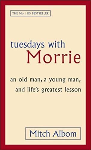
<p><img src="https://yanlin-duan.github.io/assets/pics/joining_robinhood/6.jpg" alt="Tuesdays with Morrie的封面。这是我未来manager Hongxia推荐的一本书。我在去旧金山的飞机上看完最后两章，哭成SB。" /></p>

<p><em>Tuesdays with Morrie的封面。这是我未来manager Hongxia推荐的一本书。我在去旧金山的飞机上看完最后两章，哭成SB。</em></p>

<p>虽然Kosbie说对于我找工作如此顺利收获诸多offer一点都不意外，但可能Kosbie自己都不记得的是，三年前其实我是被Kosbie“劝退”过的人。</p>

<p>那天上午我第一次走进15-112的教室。我从没去过那么大的阶梯教室。我坐在不高不低的位置，懵懵懂懂听了一整节课。我以为第一节课大概就是做一做intro，教教print Hello world，一个多小时的课上半个小时也就差不多了。没想到第一节课就这么intense。print Hello World真的只教了30秒。对，30秒。第一节课，除了所有logistic &amp; admin stuff，我们就讲了input, output, import modules, functions, return v.s. print, different types of error, variable scope…. 我记得特别清楚，当时有个同学举手问“is Python a compiled language or an interpreted language?” ，我听到的就是”is Python a bla or a bla?”，真的一脸懵逼，心想他们在说什么“鸟语”。我这个大三的“好学生”从来没有听一门课的第一节课就这么吃力过，更别提是面向大一新生的课。</p>

<p>下课了我赶紧跑去台前跟Kosbie自我介绍了一下。我说我是来CMU商学院交换一学期的交换生，这第一节课听的我很怕怕，问他选这门课适不适合我。</p>

<p>Kosbie问我，“Why do you want to take this class?” （你为什么想上这门课？）</p>

<p>我说，“Because I want to learn some programming.” （因为我想学一些编程。）</p>

<p>“If you want to learn some programming, you should go take 15-110. It’s less intense, and you may find it more fun.” （如果你只是想学一些编程的话，去上15-110吧。那个课节奏更慢些，你可能会觉得更好玩。）</p>

<p>”If 15-110 is for learning some programming, what is this class for?” （那如果15-110是教一些编程的话，这节课教什么呢？）</p>

<p>“You know, At the end of this 15-week class, students will work on an individual term project. People get Microsoft internship with it.” （在这个课上，上完这15周的课你要做一个单人的编程项目。有学生用这个项目拿到了微软的实习。）</p>

<p>大一新生。上十五周课。拿到微软实习。这是我从来没有想过的事情。 我在卡内基梅隆时写的一篇名为“纠结”的日记恰恰好描述了我当时的心境：</p>

<p>“ 
my dear diary，</p>

<p>希望我和你的对话能够帮助我搞清楚我究竟该怎么做。 
第一次对自己的能力产生了质疑。这是我想要的么？上112。似乎在这个课上做的好了可以证明我自己，但也有很大可能我做不好。 
我要花很多很多时间在这上面，但是这值得吗？ 
对于我的未来 学习这门语言的帮助 到底有多大 
我到底想要什么 
如果我不去112 是不是我就认输了？ 
是不是就代表着，我已经承认自己没有编程的天赋了？ 
112，如果学完，是可以直接出来用python找工作的 
我并不一定有机会，在我这辈子，再去学习一门编程语言 
可能就不再有机会 在CMU学习 
在CMU的这一个学期，可能是我与这所学校唯一的交集 
在这短短的一个学期里，我究竟能做什么? 
我的交换生涯的目标又是什么？？ 
我究竟需不需要在交换的这段时间 投入一切的学习它 
我能不能完成 
光是看到Term project我就觉得毫无头绪 
光是听完第一节课我就觉得有很多东西需要消化 
一周12小时，15小时甚至20小时 
仅仅投入在这一门课上 
可我还有很多很多很多事情要做</p>

<p>我真的真的有时间去完成这门课程么？ 
我不知道 
我不知道为什么现在我在纠结 
是因为我不敢确定我是否能完成它么？ 
是英语的问题？ 
数学的问题？ 
”</p>

<p>现在重读这篇日记，感觉有些中二，但又很真实。我在日记里问自己“我要花很多很多时间在这上面，但是这值得吗？”假如我有时光机，现在的我一定会不假思索的跳上它，回到2014年的8月26日，回到Morewood Garden四楼那件小小宿舍里的我的旁边，肯定的说：</p>

<p>“没有比这更值得的事情了。”</p>

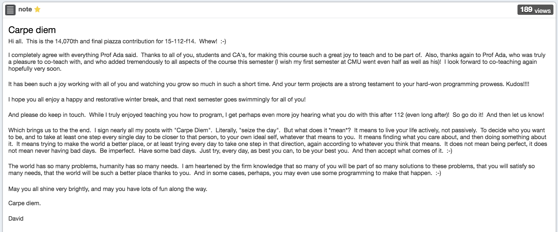
<p><img src="https://yanlin-duan.github.io/assets/pics/joining_robinhood/7.png" alt="Prof. David Kosbie在2014年秋季学期的最后一封Piazza note" />
<em>Prof. David Kosbie在2014年秋季学期的最后一封Piazza note</em></p>

<h1 id="6">6</h1>

<p>其实在我走进Robinhood办公室的一瞬间，在我内心最深处可能我已经知道自己如果拿到offer，会来这里工作了吧；当其他人问我Robinhood给我的感觉是怎样的时候，我会说：</p>

<p>一，当我进到他们办公室的时候，我就被他们的“vibe”（氛围）所吸引— 那是一种“轻松的忙碌”的状态。能听到说话的嗡嗡声，总有人在走来走去，能感觉到有很多事要做；但这种忙碌又不同于很多公司的那种很强硬很压力的忙碌，公司的氛围还是很轻松的。狗狗跑来跑去，也可以看到有同事在开心的聊天说笑。</p>

<p>二，跟面试官聊完之后，我仿佛见到了很多个“我”。大家对于做一个好的product都很有热情；工程师也很重视产品设计和用户研究；而且聊到很多问题的时候都属于双方越聊越high型。聊到激动的时候，我就直接打开airbnb的网站，给他们看哪块是我做的，我是怎么做的；或者在白板上写写画画，讲system或product的design。至于coding的部分，Robinhood也是不同于其他很多公司。问题虽不难，但要求却是要Pythonic code that can check into the production code base。我很喜欢面试官问的一针见血的问题，有些时候也让我看到了自己的思维盲点和代码方面很多值得提升的地方：我的面试官们简直就是我希望自己在几年后成为的样子。</p>

<p>Kosbie其实并没有告诉我第一份工作应该去哪里。但他说在你很难去理性选择的时候，不妨听从你的直觉。</p>

<p>我的直觉说，我属于这里。我喜欢这儿的产品，喜欢这个团队，喜欢这里充满挑战性和影响力的项目，喜欢这儿的文化。</p>

<p>那新的旅程，就从Robinhood开始吧。</p>

<p><img src="https://yanlin-duan.github.io/assets/pics/joining_robinhood/8.jpg" alt="Go Robinhood!" />
<em>Go Robinhood!</em></p>

<h1 id="7">7</h1>

<p>正如我一周前的朋友圈所说，想感谢的人有点多：</p>

<p>先感谢David Kosbie，感谢2014年秋季学期15-112的所有助教和同学，是你们一同改变了我的人生轨迹。</p>

<p>感谢我在Airbnb的manager Claire。你是我tech实习的第一个manager。谢谢你给我的所有support和candid feedback，让我可以成长的这么快！</p>

<p>感谢我在加州实习认识的所有full-time和intern小伙伴！</p>

<p>感谢SEO team！享受跟你们一起讨论买房生娃比特币的时光，还有各种trash talk XD</p>

<p>感谢“做作爆棚”的Airkill团队！作为为数不多从头跟到尾的实习生还参加了offsite特别活动。谢谢大家让我认识到了自己人生如戏戏如人生～</p>

<p>感谢上·进（a.k.a 肾群）intern小分队！谢谢你们给了我一个菠萝味的夏天 :) （大雾）</p>

<p>感谢7月4小分队！每次跟各位的旅行都是对灵魂的拷问。希望下次一起旅行的时候我可以有故事分享给大家lol</p>

<p>感谢所有跟我phone chat/内推我的朋友们，特别感激你们愿意拿出时间回答我的问题，认可并内推我！</p>

<p>感谢Rachel from Asana和Vasusen from Coursera。你们都是我特别特别欣赏的manager &amp; engineer。跟你们的聊天总是特别的有收获。没能加入你们的团队是我的遗憾。希望可以keep in touch!</p>

<p>感谢Robinhood的面试官们选择了我。Special thanks to Hongxia。以后多多指教啦！</p>

<p>感谢Yuyang学姐，Max Zhou还有易姐姐给我很多找工作+职场相关的建议！</p>

<p>感谢温总邀请我加入脑力+体力共同运动的健身小分队！各位健身达人带我举铁，我帮大家回答关于CS的各种问题，也算是”friends with benefit”了XD 谢谢你们让我两个月瘦了五公斤（希望不是累的）！</p>

<p>感谢朱总实力提供三番住宿！</p>

<p>感谢陈总实力提供匹兹堡住宿！</p>

<p>感谢戎姐在我东西海岸飞到快go die的时候carry了我的project们！</p>

<p>感谢我的粑粑麻麻支持我的决定！</p>

<p>感谢所有读到这里的你们 :)</p>]]></content><author><name>Alan Duan</name><email>duanyanl97@gmail.com</email></author><category term="Career" /><category term="Learning Diary" /><summary type="html"><![CDATA[心路历程有点长，想感谢的人有点多]]></summary></entry><entry><title type="html">My Review Note for Applied Machine Learning (Second Half)</title><link href="https://yanlin-duan.github.io/machine%20learning/cheatsheetappliedMLpart2/" rel="alternate" type="text/html" title="My Review Note for Applied Machine Learning (Second Half)" /><published>2017-04-29T00:00:00+00:00</published><updated>2017-04-29T00:00:00+00:00</updated><id>https://yanlin-duan.github.io/machine%20learning/cheatsheetappliedMLpart2</id><content type="html" xml:base="https://yanlin-duan.github.io/machine%20learning/cheatsheetappliedMLpart2/"><![CDATA[<aside class="sidebar__right">
<nav class="toc">
    <header><h4 class="nav__title"><i class="fa fa-file-text"></i> On This Page</h4></header>
<ul class="toc__menu" id="markdown-toc">
  <li><a href="#why-this-post" id="markdown-toc-why-this-post">Why this post</a></li>
  <li><a href="#acknowledgment" id="markdown-toc-acknowledgment">Acknowledgment</a></li>
  <li><a href="#model-evaluation-metrics" id="markdown-toc-model-evaluation-metrics">Model Evaluation Metrics</a>    <ul>
      <li><a href="#classification" id="markdown-toc-classification">Classification</a>        <ul>
          <li><a href="#why-do-we-need-precision-recall-and-f-score" id="markdown-toc-why-do-we-need-precision-recall-and-f-score">Why do we need precision, recall and f-score</a></li>
          <li><a href="#other-common-tools" id="markdown-toc-other-common-tools">Other common tools</a></li>
          <li><a href="#multi-class-classification-metrics" id="markdown-toc-multi-class-classification-metrics">Multi-class Classification Metrics</a></li>
        </ul>
      </li>
      <li><a href="#regression" id="markdown-toc-regression">Regression</a>        <ul>
          <li><a href="#built-in-standard-metrics" id="markdown-toc-built-in-standard-metrics">Built-in standard metrics</a></li>
        </ul>
      </li>
      <li><a href="#clustering-supervised-evaluation" id="markdown-toc-clustering-supervised-evaluation">Clustering (supervised evaluation)</a>        <ul>
          <li><a href="#why-cant-we-use-accuracy-score" id="markdown-toc-why-cant-we-use-accuracy-score">Why can’t we use accuracy score</a></li>
          <li><a href="#contigency-matrix" id="markdown-toc-contigency-matrix">Contigency matrix</a></li>
          <li><a href="#rand-index-adjusted-rand-index-normalized-mutual-information-and-adjusted-mutual-information" id="markdown-toc-rand-index-adjusted-rand-index-normalized-mutual-information-and-adjusted-mutual-information">Rand Index, Adjusted Rand Index, Normalized Mutual Information and Adjusted Mutual Information</a></li>
        </ul>
      </li>
      <li><a href="#clustering-unsupervised-evaluation" id="markdown-toc-clustering-unsupervised-evaluation">Clustering (unsupervised evaluation)</a>        <ul>
          <li><a href="#silhouette-score" id="markdown-toc-silhouette-score">Silhouette Score</a></li>
        </ul>
      </li>
      <li><a href="#sample-code-for-choosing-evaluation-metrics-in-sklearn" id="markdown-toc-sample-code-for-choosing-evaluation-metrics-in-sklearn">Sample code for choosing evaluation metrics in sklearn</a></li>
    </ul>
  </li>
  <li><a href="#dimensionality-reduction" id="markdown-toc-dimensionality-reduction">Dimensionality Reduction</a>    <ul>
      <li><a href="#linear-unsupervised-transformation--pca" id="markdown-toc-linear-unsupervised-transformation--pca">Linear, Unsupervised Transformation – PCA</a>        <ul>
          <li><a href="#why-pca-in-general-works" id="markdown-toc-why-pca-in-general-works">Why PCA (in general) works</a></li>
          <li><a href="#important-notes" id="markdown-toc-important-notes">Important notes</a></li>
          <li><a href="#sample-code" id="markdown-toc-sample-code">Sample Code</a></li>
        </ul>
      </li>
      <li><a href="#unsupervised-transformation--nmf" id="markdown-toc-unsupervised-transformation--nmf">Unsupervised Transformation – NMF</a></li>
      <li><a href="#non-linear-unsupervised-transformation---t-sne" id="markdown-toc-non-linear-unsupervised-transformation---t-sne">Non-linear, unsupervised transformation - t-SNE</a>        <ul>
          <li><a href="#note" id="markdown-toc-note">Note</a></li>
        </ul>
      </li>
      <li><a href="#linear-supervised-transformation--linear-discriminant-analysis" id="markdown-toc-linear-supervised-transformation--linear-discriminant-analysis">Linear, supervised transformation – Linear Discriminant Analysis</a></li>
    </ul>
  </li>
  <li><a href="#outlier-detection" id="markdown-toc-outlier-detection">Outlier detection</a>    <ul>
      <li><a href="#elliptic-envelope" id="markdown-toc-elliptic-envelope">Elliptic Envelope</a></li>
      <li><a href="#kernel-density" id="markdown-toc-kernel-density">Kernel Density</a></li>
      <li><a href="#one-class-svm" id="markdown-toc-one-class-svm">One class SVM</a></li>
      <li><a href="#isolation-forests" id="markdown-toc-isolation-forests">Isolation Forests</a>        <ul>
          <li><a href="#normalizing-path-length" id="markdown-toc-normalizing-path-length">Normalizing path length</a></li>
          <li><a href="#building-the-forest" id="markdown-toc-building-the-forest">Building the forest</a></li>
        </ul>
      </li>
    </ul>
  </li>
  <li><a href="#working-with-imbalanced-data" id="markdown-toc-working-with-imbalanced-data">Working with imbalanced data</a>    <ul>
      <li><a href="#change-threshold" id="markdown-toc-change-threshold">Change threshold</a></li>
      <li><a href="#sampling-approaches" id="markdown-toc-sampling-approaches">Sampling approaches</a>        <ul>
          <li><a href="#random-undersampling" id="markdown-toc-random-undersampling">Random undersampling</a></li>
          <li><a href="#random-oversampling" id="markdown-toc-random-oversampling">Random oversampling</a></li>
          <li><a href="#class-weights" id="markdown-toc-class-weights">Class-weights</a></li>
          <li><a href="#ensemble-resampling" id="markdown-toc-ensemble-resampling">Ensemble resampling</a></li>
          <li><a href="#edited-nearest-neighbors" id="markdown-toc-edited-nearest-neighbors">Edited Nearest Neighbors</a></li>
          <li><a href="#condensed-nearest-neighbors" id="markdown-toc-condensed-nearest-neighbors">Condensed Nearest Neighbors</a></li>
          <li><a href="#synthetic-minority-oversampling-technique-smote" id="markdown-toc-synthetic-minority-oversampling-technique-smote">Synthetic Minority Oversampling Technique (SMOTE)</a></li>
        </ul>
      </li>
    </ul>
  </li>
  <li><a href="#clustering-and-mixture-model" id="markdown-toc-clustering-and-mixture-model">Clustering and Mixture Model</a>    <ul>
      <li><a href="#k-means-algorithm" id="markdown-toc-k-means-algorithm">K-Means algorithm</a></li>
      <li><a href="#agglomerative-clustering" id="markdown-toc-agglomerative-clustering">Agglomerative clustering</a></li>
      <li><a href="#dbscan" id="markdown-toc-dbscan">DBSCAN</a></li>
      <li><a href="#mixture-models" id="markdown-toc-mixture-models">Mixture Models</a></li>
      <li><a href="#bayesian-infinite-mixtures" id="markdown-toc-bayesian-infinite-mixtures">Bayesian Infinite Mixtures</a></li>
      <li><a href="#a-zoo-of-clustering-algorithm-" id="markdown-toc-a-zoo-of-clustering-algorithm-">A zoo of clustering algorithm </a></li>
      <li><a href="#on-picking-the-correct-number-of-clusters" id="markdown-toc-on-picking-the-correct-number-of-clusters">On picking the “correct” number of clusters</a>        <ul>
          <li><a href="#silhouette-plots-" id="markdown-toc-silhouette-plots-">Silhouette Plots </a></li>
          <li><a href="#cluster-stability" id="markdown-toc-cluster-stability">Cluster Stability</a></li>
          <li><a href="#qualitative-evaluation-fancy-name-for-eyeballing" id="markdown-toc-qualitative-evaluation-fancy-name-for-eyeballing">Qualitative Evaluation (Fancy name for eyeballing)</a></li>
          <li><a href="#gridsearchcv-if-doing-feature-extraction" id="markdown-toc-gridsearchcv-if-doing-feature-extraction">GridSearchCV (if doing feature extraction)</a></li>
        </ul>
      </li>
    </ul>
  </li>
  <li><a href="#natural-language-processing" id="markdown-toc-natural-language-processing">Natural Language Processing</a>    <ul>
      <li><a href="#generating-features-from-text" id="markdown-toc-generating-features-from-text">Generating features from text</a>        <ul>
          <li><a href="#tokenization" id="markdown-toc-tokenization">Tokenization</a></li>
          <li><a href="#normalization-preprocessing" id="markdown-toc-normalization-preprocessing">Normalization (preprocessing)</a></li>
          <li><a href="#restricting-the-vocabulary-feature-selection" id="markdown-toc-restricting-the-vocabulary-feature-selection">Restricting the vocabulary (feature selection)</a></li>
          <li><a href="#beyond-unigram-feature-engineering" id="markdown-toc-beyond-unigram-feature-engineering">Beyond unigram (Feature engineering)</a></li>
          <li><a href="#large-scale-text-vectorization--hashing" id="markdown-toc-large-scale-text-vectorization--hashing">Large scale text vectorization – hashing</a></li>
          <li><a href="#beyond-bag-of-words" id="markdown-toc-beyond-bag-of-words">Beyond Bag of Words</a></li>
          <li><a href="#word-embedding" id="markdown-toc-word-embedding">Word embedding</a></li>
        </ul>
      </li>
    </ul>
  </li>
  <li><a href="#neural-networks" id="markdown-toc-neural-networks">Neural Networks</a>    <ul>
      <li><a href="#general-architecture" id="markdown-toc-general-architecture">General architecture</a></li>
      <li><a href="#back-propagation" id="markdown-toc-back-propagation">Back-propagation</a></li>
      <li><a href="#solvers" id="markdown-toc-solvers">Solvers</a></li>
      <li><a href="#complexity-control" id="markdown-toc-complexity-control">Complexity control</a></li>
      <li><a href="#autodiff" id="markdown-toc-autodiff">Autodiff</a></li>
      <li><a href="#calculate-number-of-parameters-in-neural-network" id="markdown-toc-calculate-number-of-parameters-in-neural-network">Calculate number of parameters in neural network</a></li>
      <li><a href="#keras" id="markdown-toc-keras">Keras</a>        <ul>
          <li><a href="#note-1" id="markdown-toc-note-1">Note</a></li>
          <li><a href="#necessary-preparation" id="markdown-toc-necessary-preparation">Necessary preparation</a></li>
          <li><a href="#code" id="markdown-toc-code">Code</a></li>
        </ul>
      </li>
      <li><a href="#drop-out-regularization" id="markdown-toc-drop-out-regularization">Drop-out regularization</a>        <ul>
          <li><a href="#code-1" id="markdown-toc-code-1">Code</a></li>
        </ul>
      </li>
      <li><a href="#convolutional-neural-network" id="markdown-toc-convolutional-neural-network">Convolutional Neural Network</a>        <ul>
          <li><a href="#how-many-neurons-fit-in-each-layer-" id="markdown-toc-how-many-neurons-fit-in-each-layer-">How many neurons fit in each layer </a></li>
          <li><a href="#parameter-sharing" id="markdown-toc-parameter-sharing">Parameter Sharing</a></li>
          <li><a href="#max-pooling" id="markdown-toc-max-pooling">Max pooling</a></li>
          <li><a href="#batch-normalization" id="markdown-toc-batch-normalization">Batch Normalization</a></li>
          <li><a href="#use-pre-trained-networks" id="markdown-toc-use-pre-trained-networks">Use pre-trained networks</a></li>
          <li><a href="#adverserial-samples" id="markdown-toc-adverserial-samples">Adverserial Samples</a></li>
        </ul>
      </li>
    </ul>
  </li>
  <li><a href="#time-series" id="markdown-toc-time-series">Time Series</a>    <ul>
      <li><a href="#tasks" id="markdown-toc-tasks">Tasks</a></li>
      <li><a href="#parse-date--time-series-index" id="markdown-toc-parse-date--time-series-index">Parse date &amp; Time Series Index</a></li>
      <li><a href="#backfil-and-forward-fill" id="markdown-toc-backfil-and-forward-fill">Backfil and forward fill</a></li>
      <li><a href="#resampling" id="markdown-toc-resampling">Resampling</a></li>
      <li><a href="#detrending-look-at-differencing" id="markdown-toc-detrending-look-at-differencing">Detrending (look at differencing)</a></li>
      <li><a href="#autocorrelation-correlation-between-two-data-point" id="markdown-toc-autocorrelation-correlation-between-two-data-point">Autocorrelation (correlation between two data point)</a></li>
      <li><a href="#autoregressive-linear-model" id="markdown-toc-autoregressive-linear-model">Autoregressive linear model</a></li>
      <li><a href="#arima" id="markdown-toc-arima">ARIMA</a></li>
      <li><a href="#with-scikit-learn-fit-linearquadratic-linear-regression" id="markdown-toc-with-scikit-learn-fit-linearquadratic-linear-regression">With scikit-learn: fit linear/quadratic linear regression</a></li>
      <li><a href="#side-note-pandas-group-by-function" id="markdown-toc-side-note-pandas-group-by-function">Side note: pandas group-by function</a></li>
    </ul>
  </li>
</ul>

  </nav>
</aside>

<h1 id="why-this-post">Why this post</h1>

<p>This semester I am taking Applied Machine Learning with <a href="http://amueller.github.io/">Andreas Mueller</a>. It’s a great class focusing on the practical side of machine learning.</p>

<p>I received many positive feedbacks for my review note of the first half of the class. I am therefore motivated to continue working on a similar post for the second half. Again, I am posting my notes on my blog so it can benefit more people, no matter he/she is in the class or not :)</p>

<h1 id="acknowledgment">Acknowledgment</h1>

<p>The texts of this note are largely inspired by:</p>

<ul>
  <li><a href="https://amueller.github.io/applied_ml_spring_2017/">Course material</a> for COMS 4995 Applied Machine Learning.</li>
</ul>

<p>The example codes in this note are modified based on:</p>

<ul>
  <li><a href="https://amueller.github.io/applied_ml_spring_2017/">Course material</a> for COMS 4995 Applied Machine Learning.</li>
  <li>Supplemental material of <em>An Introduction to Machine Learning with Python</em> by Andreas C. Müller and Sarah Guido (O’Reilly). Copyright 2017 Sarah Guido and Andreas Müller, 978-1-449-36941-5.</li>
</ul>

<p>Care has been taken to avoid copyrighted contents as much as possible, and give citation wherever is proper.</p>

<h1 id="model-evaluation-metrics">Model Evaluation Metrics</h1>

<h2 id="classification">Classification</h2>

<h3 id="why-do-we-need-precision-recall-and-f-score">Why do we need precision, recall and f-score</h3>

<p>It is very natural to evaluate the performance of a model by looking at its <strong>accuracy</strong> – meaning out of all testing data, how many we get <em>correct</em> (predict true when it should be true, and predict false when it should be false).</p>

<p>However, this measurement becomes less effective if the data is imbalanced – meaning we have way more data in one class compared to others. For example – if 99% of the data are labeled as 1, a model can simply “cheat” by always predicting 1 – a naive, trivial but high accuracy model. In those cases, we need better measurements, and that’s why we introduce precision and recall.</p>

<p>I have had a long time memorizing which one is which, and there are so many combinations between True Positive, False Positive, True Negative and False Negative so I almost always get confused. I found it’s actually easier if we take a step back and first intuitively understand the word “precision” and “recall” (yes, the name is not a random one!)</p>

<p>When we say precision, we are talking about how precise you are. For example, if I am searching something on Google, I will say the precision is high when <em>out of everything Google returns to me</em>, I found most of them relevant to what I want to search for.</p>

<p>This means, I am measuring the proportion of correct search results (True positive) over everything Google predicts to be “what I want” (True positive and False positive).</p>

<p>For recall, I find it easier to understand it in an “ecology” context – in ecology, there is a method called <strong>“mark and recapture”</strong> where a portion of the population of, say, an insect is captured, marked and released (we remember how many we marked). Later, another portion is captured. We are now interested in <strong>out of all the marked insects</strong>, how much do we recall.</p>

<p>Back to machine learning, this naturally translates to the proportion of <em>“recaptured and marked ones”</em> (true positive) over <em>all marked insects</em> (true positive + false negative, i.e. those mark insects we recapture + fail to recapture).</p>

<p><strong>Sanity Check time: if this review note is to predict topics covered in class, what should I include if I want to have a high precision? (Hint: count # of parameters in a neural network) How about a high recall?</strong></p>

<p>As you can see from the sanity check question, it is not hard for models to achieve a perfect recall or a perfect precision <em>alone</em>. Therefore, we would like to summarize them – and that’s what f-score, the harmonic mean of precision and recall, is doing.</p>

<h3 id="other-common-tools">Other common tools</h3>

<ul>
  <li>
    <p>Precision-Recall Curve. Area under it is the <strong>average precision</strong> (ignoring some technical differences). Ideal curve –upper right.</p>
  </li>
  <li>
    <p>Receiver operating characterisitics (ROC), which is FPR (\(FP/(FP+TN)\))v.s. TPR (recall). AUC is the area under the curve, which does not depend on threshold selection. AUC is always 0.5 for random prediction, regardless of whether the class is balanced. The AUC can be interpreted as evaluating the ranking of positive samples. Ideal curve – upper left.</p>
  </li>
</ul>

<h3 id="multi-class-classification-metrics">Multi-class Classification Metrics</h3>

<ul>
  <li>Confusion Matrix and classification report (note: support means  number of data points (ground truth) in that class)</li>
  <li>Micro-F1 (each data point to be equal weight) and Macro-F1 (each class to be equal weight)</li>
</ul>

<h2 id="regression">Regression</h2>

<h3 id="built-in-standard-metrics">Built-in standard metrics</h3>

<ul>
  <li>\(R^2\): a standardized measure of degree of predictedness, or fit, in the sample. Easy to understand scale.</li>
  <li>MSE: estimate the variance of residuals, or non-fit, in the population. Easy to relate to input</li>
  <li>Mean Absolute Error, Median Absolute Error, Mean Absolute Percentage Error etc.</li>
  <li>\(R^2\) is still the most commonly used one.</li>
</ul>

<h2 id="clustering-supervised-evaluation">Clustering (supervised evaluation)</h2>

<p>When evaluating clustering with the ground truth, note that labels do not matter – [0,1,0,1] is exactly the same as [1,0,1,0]. We should only look at <strong>partition</strong>.</p>

<h3 id="why-cant-we-use-accuracy-score">Why can’t we use accuracy score</h3>

<p>The problem in using accuracy in clustering problem is that it requires <em>exactly match</em> between the ground truth and the predicted label. However, the cluster labels themselves are meaningless – as mentioned above, we should only care about partition, not labels!</p>

<h3 id="contigency-matrix">Contigency matrix</h3>
<p>One tool we will use is contingency matrix. It is similar as confusion matrix, except that it does not have to square, and switching of rows/columns will not change the result.</p>

<h3 id="rand-index-adjusted-rand-index-normalized-mutual-information-and-adjusted-mutual-information">Rand Index, Adjusted Rand Index, Normalized Mutual Information and Adjusted Mutual Information</h3>

<p>Rand index measures the similarity between two clustering. The formula is \(RI(C_1,C_2) = \frac{a+b}{n \choose 2}\), where \(a\) is the number of pairs of points that are in the same set in both cluster \(C_1\) and \(C_2\), while $b$ is the number of pairs of points that are in different sets in $C_1$ and $C_2$. The denominator is just number of all possible pairs.</p>

<p>It can be intuitively understood if we view each pair as a data point, and treat this problem as using \(C_2\) to predict \(C_1\) (the ground truth). (Or the other way around, it’s symmetric).</p>

<p>We count the number of true positive (they are in the same cluster in \(C_1\), and \(C_2\) predicts that they are also in a same cluster), plus the number of true negative (they are not in the same cluster in \(C_1\), and \(C_2\) predicts that they are also not in a same cluster) Sounds familiar now? Yes, it is just an analogy of accuracy!</p>

<p><strong>Sanity Check Question: What is R([0,1,0,1], [1,0,0,2])?</strong></p>

<p>Rand Index always ranges between 0 and 1. The bigger the better.</p>

<p>Adjusted Rand Index (ARI) is introduced to ensure to have a value close to 0.0 for random labeling independently of the number of clusters and samples and exactly 1.0 when the clusterings are identical (up to a permutation). <strong>ARI penalizes too many clusters</strong>. <strong>ARI can become negative</strong>.</p>

<p>Note: ARI requires the knowledge of ground truth. Therefore, <strong>ARI is not a practical way to assess clustering algorithms like K-Means.</strong></p>

<p>Furthermore, we have normalized mutual information (which penalizes overpatitions via entropy) and adjusted mutual information (adjust for chance, so any two random partitions have expected AMI of 0).</p>

<h2 id="clustering-unsupervised-evaluation">Clustering (unsupervised evaluation)</h2>

<h3 id="silhouette-score">Silhouette Score</h3>

<p>Formula:</p>

<p>For each sample, calculate \(s = \frac{b-a}{\max(a,b)}\), where \(a\) is mean distance to samples in same cluster, \(b\) is the mean distance to samples in nearest cluster.</p>

<p>For whole clustering, we average s over all samples.</p>

<p>This scoring prefers compact clusters (like K-means).</p>

<p>Rationale: we want to maximize the difference between \(b\) and \(a\), so that the result is <em>decoupling and cohesion</em> (sounds like object-oriented programming hah?)</p>

<p>Cons: While compact clusters are good, compactness doesn’t allow for complex shapes.</p>

<h2 id="sample-code-for-choosing-evaluation-metrics-in-sklearn">Sample code for choosing evaluation metrics in sklearn</h2>

<div class="language-python highlighter-rouge"><div class="highlight"><pre class="highlight"><code><span class="c1"># default scoring for classification is accuracy
</span><span class="n">scores_default</span> <span class="o">=</span> <span class="n">cross_val_score</span><span class="p">(</span><span class="n">SVC</span><span class="p">(),</span> <span class="n">X</span><span class="p">,</span> <span class="n">y</span><span class="p">)</span>

<span class="c1"># providing scoring="accuracy" doesn't change the results
</span><span class="n">explicit_accuracy</span> <span class="o">=</span>  <span class="n">cross_val_score</span><span class="p">(</span><span class="n">SVC</span><span class="p">(),</span> <span class="n">X</span><span class="p">,</span> <span class="n">y</span><span class="p">,</span> <span class="n">scoring</span><span class="o">=</span><span class="s">"accuracy"</span><span class="p">)</span>

<span class="c1"># using ROC AUC
</span><span class="n">roc_auc</span> <span class="o">=</span>  <span class="n">cross_val_score</span><span class="p">(</span><span class="n">SVC</span><span class="p">(),</span> <span class="n">X</span><span class="p">,</span> <span class="n">digits</span><span class="p">.</span><span class="n">target</span> <span class="o">==</span> <span class="mi">9</span><span class="p">,</span> <span class="n">scoring</span><span class="o">=</span><span class="s">"roc_auc"</span><span class="p">)</span>

<span class="c1"># Implement your own scoring function
</span><span class="k">def</span> <span class="nf">few_support_vectors</span><span class="p">(</span><span class="n">est</span><span class="p">,</span> <span class="n">X</span><span class="p">,</span> <span class="n">y</span><span class="p">):</span>
    <span class="n">acc</span> <span class="o">=</span> <span class="n">est</span><span class="p">.</span><span class="n">score</span><span class="p">(</span><span class="n">X</span><span class="p">,</span> <span class="n">y</span><span class="p">)</span>
    <span class="n">frac_sv</span> <span class="o">=</span> <span class="nb">len</span><span class="p">(</span><span class="n">est</span><span class="p">.</span><span class="n">support_</span><span class="p">)</span> <span class="o">/</span> <span class="n">np</span><span class="p">.</span><span class="nb">max</span><span class="p">(</span><span class="n">est</span><span class="p">.</span><span class="n">support_</span><span class="p">)</span>
    <span class="c1"># I just made this up, don't actually use this
</span>    <span class="k">return</span> <span class="n">acc</span> <span class="o">/</span> <span class="n">frac_sv</span>

<span class="n">param_grid</span> <span class="o">=</span> <span class="p">{</span><span class="s">'C'</span><span class="p">:</span> <span class="n">np</span><span class="p">.</span><span class="n">logspace</span><span class="p">(</span><span class="o">-</span><span class="mi">3</span><span class="p">,</span> <span class="mi">2</span><span class="p">,</span> <span class="mi">6</span><span class="p">)}</span>
<span class="n">grid</span> <span class="o">=</span> <span class="n">GridSearchCV</span><span class="p">(</span><span class="n">SVC</span><span class="p">(),</span> <span class="n">param_grid</span><span class="o">=</span><span class="n">param_grid</span><span class="p">,</span> <span class="n">cv</span><span class="o">=</span><span class="mi">10</span><span class="p">,</span> <span class="n">scoring</span><span class="o">=</span><span class="n">few_support_vectors</span><span class="p">)</span>
</code></pre></div></div>

<h1 id="dimensionality-reduction">Dimensionality Reduction</h1>

<h2 id="linear-unsupervised-transformation--pca">Linear, Unsupervised Transformation – PCA</h2>

<p>PCA rotates the dataset so that the rotated features are statistically uncorrelated. It first finds the direction of maximum variance, and then finds the direction that has maximum variance but at the same time <strong>is orthogonal</strong> to the first direction (thus making those two rotated features not correlated), so on and so forth.</p>

<p>When to use: PCA is commonly used for linear dimension reduction (select up to first k principal components), visualization of high-dimensional data (draw first v.s. second principal components), regularization and feature extraction (for example, comparing distance in pixel space does not really make sense; maybe using PCA space will perform better)</p>

<p>Whitening: rescale the principal components to have the same scale; Same as using StandardScaler after perfoming PCA.</p>

<h3 id="why-pca-in-general-works">Why PCA (in general) works</h3>

<p>PCA finds uncorrelated components that maximizes the variance explained in the data. However, only when the data follows Gaussian distribution, zero correlation between components implies independence, as the first and second order statistics already captures all the information. This is not true for most of the other distributions.</p>

<p>Therefore, PCA ‘sort of’ makes an implicit assumption that data is drawn from Gaussian, and works the best when representing multivariate normally distributed data.</p>

<h3 id="important-notes">Important notes</h3>

<ul>
  <li>PCA, compared to histograms or other tools, is used because it can capture the interactions between features.</li>
  <li>Do scaling before performing PCA. Imagine one feature with very large scale. Without scaling, it’s guaranteed to be the first principal component!</li>
  <li>PCA is unsupervised, so it does not use any class information.</li>
  <li>PCA has no guarantee that the top k principal components are the dimensions that <strong>contains most information</strong>. High variance \(!=\) most information!</li>
  <li>Max number of principal components min(n_samples, n_features).</li>
  <li>Sign of the principal components does not mean <strong>anything</strong>.</li>
  <li>There’s cancellation effects because of the negative components.</li>
</ul>

<h3 id="sample-code">Sample Code</h3>

<div class="language-python highlighter-rouge"><div class="highlight"><pre class="highlight"><code><span class="n">pca_lr</span> <span class="o">=</span> <span class="n">make_pipeline</span><span class="p">(</span><span class="n">StandardScaler</span><span class="p">(),</span> <span class="n">PCA</span><span class="p">(</span><span class="n">n_components</span><span class="o">=</span><span class="mi">2</span><span class="p">),</span> <span class="n">LogisticRegression</span><span class="p">(</span><span class="n">C</span><span class="o">=</span><span class="mi">1</span><span class="p">))</span>
<span class="n">pca_lr</span><span class="p">.</span><span class="n">fit</span><span class="p">(</span><span class="n">X_train</span><span class="p">,</span> <span class="n">y_train</span><span class="p">)</span>

<span class="n">pca</span> <span class="o">=</span> <span class="n">PCA</span><span class="p">(</span><span class="n">n_components</span><span class="o">=</span><span class="mi">100</span><span class="p">,</span> <span class="n">whiten</span><span class="o">=</span><span class="bp">True</span><span class="p">,</span> <span class="n">random_state</span><span class="o">=</span><span class="mi">0</span><span class="p">).</span><span class="n">fit</span><span class="p">(</span><span class="n">X_train</span><span class="p">)</span>
<span class="n">X_train_pca</span> <span class="o">=</span> <span class="n">pca</span><span class="p">.</span><span class="n">transform</span><span class="p">(</span><span class="n">X_train</span><span class="p">)</span>
<span class="n">X_test_pca</span> <span class="o">=</span> <span class="n">pca</span><span class="p">.</span><span class="n">transform</span><span class="p">(</span><span class="n">X_test</span><span class="p">)</span>
</code></pre></div></div>

<h2 id="unsupervised-transformation--nmf">Unsupervised Transformation – NMF</h2>

<p>NMF stands for non-negative matrix factorization. It is similar to PCA in the sense that it is also a linear, unsupervised transformation. But instead of requiring each componenet to be orthogonal, we want the coefficients to be non-negative in NMF. Therefore, NMF only works to data where each feature is non-negative.</p>

<p>Pros:</p>

<ul>
  <li>NMF leads to more interpretable components than PCA</li>
  <li>No cancellation effect like PCA</li>
  <li>No sign ambiguity like in PCA</li>
  <li>Can learn over-complete representation (components more than features) by asking for sparsity</li>
  <li>Can be vised as a soft clustering</li>
  <li>Traditional Nonnegative Matrix Factorization (NMF) is a linear and unsupervised algorithm. But there are novice ones that can extract non-linear features (http://ieeexplore.ieee.org/document/7396284/?reload=true)</li>
</ul>

<p>Cons:</p>
<ul>
  <li>Only works on non-negative data</li>
  <li>Can be slow on large datasets</li>
  <li>Coefficients not orthogonal</li>
  <li>Components in NMF are not ordered – all play an equal part (also can be a pro)</li>
  <li>Number of components totally change the set of components.</li>
  <li>Non-convex optimization; Randomness involved in initialization</li>
</ul>

<p>Other matrix factorizations:</p>
<ul>
  <li>Sparse PCA: components orthogonal &amp; sparse</li>
  <li>ICA: independent components</li>
</ul>

<h2 id="non-linear-unsupervised-transformation---t-sne">Non-linear, unsupervised transformation - t-SNE</h2>

<p>t-distributed stochastic neighbor embedding (t-SNE) is an algorithm in the category of manifold learning. The high level idea of t-SNE is that it will find a two-dimensional representation of the data such that if they are ‘similar’ in high-dimension, they will be ‘closer’ in the reduced 2D space. To put it in another way, it tries to preserve the neighborhood information.</p>

<p>How t-SNE works: it starts with a random embedding, and iteratively updates points to make close points close.</p>

<p>The usage for t-SNE is now more on data visualization.</p>

<h3 id="note">Note</h3>
<ul>
  <li>t-SNE does not support transforming new data, so no transform method in sklearn</li>
  <li>Axes do not correspond to anything in the input space, so merely for visualization purpose.</li>
  <li>To tune t-SNE, tune perplexity (low perplxity == only close neighbors) and early_exaggeration parameters, though the effects are usually minor.</li>
</ul>

<h2 id="linear-supervised-transformation--linear-discriminant-analysis">Linear, supervised transformation – Linear Discriminant Analysis</h2>

<p><img src="http://sebastianraschka.com/images/blog/2014/linear-discriminant-analysis/lda_1.png" alt="Comparison Between PCA and LDA" /> <sup id="fnref:1" role="doc-noteref"><a href="#fn:1" class="footnote" rel="footnote">1</a></sup></p>

<p>Linear Discriminant Analysis is a “supervised” generative model that computes the directions (“linear discriminants”) that will maximize the separation between multiple classes. LDA assumes data to be drawn from Gaussian distributions (just as PCA, but for each class). It further assumes that features are statistically independent, and identical covariance matrices for every class.</p>

<p>LDA can be used both as a classifier and a dimensionality reduction techinique. The advantage is that it is a supervised model, and there’s no parameters to tune. It is also very fast since it only needs to compute means and invert covariance matrices (if number of features is way less than number of samples).</p>

<p>A variation is Quadratic Discriminant Analaysis, where basically each class will have separate covariance matrices.</p>

<h1 id="outlier-detection">Outlier detection</h1>

<h2 id="elliptic-envelope">Elliptic Envelope</h2>

<p>Assumption:</p>

<p>Data come from a known distribution (for example, Gaussian distribution).</p>

<p>Rationale: 
Define the “shape” of the data, and can define outlying observations as observations which stand far enough from the fit shape.</p>

<p>Implementation:</p>
<ul>
  <li>estimate the inlier location and covariance in a robust way (i.e. whithout being influenced by outliers).</li>
  <li>The <a href="https://en.wikipedia.org/wiki/Mahalanobis_distance">Mahalanobis distances</a> obtained from this estimate is then used to derive a measure of outlyingness.</li>
</ul>

<p>Note:</p>
<ul>
  <li>Only works if Gaussian assumption is reasonable</li>
  <li>Preprocessing with PCA might help</li>
</ul>

<h2 id="kernel-density">Kernel Density<sup id="fnref:4" role="doc-noteref"><a href="#fn:4" class="footnote" rel="footnote">2</a></sup></h2>

<p><img src="https://yanlin-duan.github.io/assets/pics/Kernel-Density-EstimationKDE.png" alt="Kernel density vs Histogram" /></p>

<p>Kernel density estimation is a non-parametric density model. Essentially it is a natural extension of histogram. The density function for histogram is not smooth, and it can be largely affected by the width of the bin. Finally, histogram won’t work with high-dimension data – all these problems can be addressed by kernel density estimation.</p>

<p>Code:</p>

<div class="language-python highlighter-rouge"><div class="highlight"><pre class="highlight"><code><span class="n">kde</span> <span class="o">=</span> <span class="n">KernelDensity</span><span class="p">(</span><span class="n">bandwidth</span><span class="o">=</span><span class="mi">3</span><span class="p">)</span>
<span class="n">kde</span><span class="p">.</span><span class="n">fit</span><span class="p">(</span><span class="n">X</span><span class="p">)</span>
<span class="n">pred</span> <span class="o">=</span> <span class="n">kde</span><span class="p">.</span><span class="n">score_samples</span><span class="p">(</span><span class="n">X_test</span><span class="p">)</span>
</code></pre></div></div>

<h2 id="one-class-svm">One class SVM</h2>

<p>One class SVM also uses Gaussian kernel to cover data. It requires the choice of a kernel and a scalar parameter to define a frontier. The RBF kernel is usually chosen as the kernel. The \(\nu\) parameter, also known as the margin of the One-Class SVM (percentage of training mistakes), corresponds to the probability of finding a new, but regular, observation outside the frontier.</p>

<p>Note:</p>

<p>As usual for SVM, do standard scaler before applying OneClassSVM is common practice.</p>

<p>Code:</p>

<div class="language-python highlighter-rouge"><div class="highlight"><pre class="highlight"><code><span class="kn">from</span> <span class="nn">sklearn.svm</span> <span class="kn">import</span> <span class="n">OneClassSVM</span>
<span class="n">oneclass</span> <span class="o">=</span> <span class="n">OneClassSVM</span><span class="p">(</span><span class="n">nu</span><span class="o">=</span><span class="mf">0.1</span><span class="p">).</span><span class="n">fit</span><span class="p">(</span><span class="n">X</span><span class="p">)</span>
<span class="n">pred</span> <span class="o">=</span> <span class="n">oneclass</span><span class="p">.</span><span class="n">predict</span><span class="p">(</span><span class="n">X_test</span><span class="p">).</span><span class="n">astype</span><span class="p">(</span><span class="n">np</span><span class="p">.</span><span class="nb">int</span><span class="p">)</span>
</code></pre></div></div>

<h2 id="isolation-forests">Isolation Forests</h2>

<p>The idea is to build a random tree and we expect that outliers are easier to isolate from the rest, since it is alone. Then we consider the path length for isolating each data point to determine who’s the outlier.</p>

<h3 id="normalizing-path-length">Normalizing path length</h3>

\[c(n) = 2H(n-1) - (2(n-1)/n)\]

<p>\(s(x,n) = 2^{-\frac{E(h(x))}{c(n)}}\), where \(h\) is the depth of the tree.</p>

<p>s close to 1 meaning it is likely to be outlier.</p>

<h3 id="building-the-forest">Building the forest</h3>

<ul>
  <li>Subsample dataset for each tree</li>
  <li>Default sample size of 256 works surprisingly well</li>
  <li>Stop growing tree at depth \(\log_2{n}\) –- so 8 No bootstrapping usually</li>
  <li>The more trees the better (default is 100 trees)</li>
  <li>Need to specify contamination rate (float in 0 to 0.5), default 0.1.</li>
</ul>

<p>Code:</p>

<div class="language-python highlighter-rouge"><div class="highlight"><pre class="highlight"><code><span class="kn">from</span> <span class="nn">sklearn.ensemble</span> <span class="kn">import</span> <span class="n">IsolationForest</span>
<span class="n">clf</span> <span class="o">=</span> <span class="n">IsolationForest</span><span class="p">(</span><span class="n">max_samples</span><span class="o">=</span><span class="mi">100</span><span class="p">,</span> <span class="n">random_state</span><span class="o">=</span><span class="mi">4</span><span class="p">,</span> <span class="n">contamination</span><span class="o">=</span><span class="mf">0.05</span><span class="p">)</span>
<span class="n">clf</span><span class="p">.</span><span class="n">fit</span><span class="p">(</span><span class="n">X_train</span><span class="p">)</span>
<span class="n">y_pred_train</span> <span class="o">=</span> <span class="n">clf</span><span class="p">.</span><span class="n">predict</span><span class="p">(</span><span class="n">X_train</span><span class="p">)</span>
</code></pre></div></div>

<h1 id="working-with-imbalanced-data">Working with imbalanced data</h1>

<h2 id="change-threshold">Change threshold</h2>

<div class="language-python highlighter-rouge"><div class="highlight"><pre class="highlight"><code><span class="n">y_pred</span> <span class="o">=</span> <span class="n">lr</span><span class="p">.</span><span class="n">predict_proba</span><span class="p">(</span><span class="n">X_test</span><span class="p">)[:,</span> <span class="mi">1</span><span class="p">]</span> <span class="o">&gt;</span> <span class="p">.</span><span class="mi">85</span> <span class="c1"># change threshold to 0.85
</span></code></pre></div></div>

<p><strong>Sanity check question: for the above code, would you expect the precision of predicting positive (class 1) to increase or decrease? How about recall? How about support?</strong></p>

<h2 id="sampling-approaches">Sampling approaches</h2>

<h3 id="random-undersampling">Random undersampling</h3>

<p>Drop data from the majority class randomly, until balanced.</p>

<p>Pros: very fast training, really good for large datasets</p>

<p>Cons: Loses data</p>

<div class="language-python highlighter-rouge"><div class="highlight"><pre class="highlight"><code><span class="kn">from</span> <span class="nn">imblearn.under_sampling</span> <span class="kn">import</span> <span class="n">RandomUnderSampler</span>

<span class="n">rus</span> <span class="o">=</span> <span class="n">RandomUnderSampler</span><span class="p">(</span><span class="n">replacement</span> <span class="o">=</span> <span class="bp">False</span><span class="p">)</span>
<span class="n">X_train_subsample</span><span class="p">,</span> <span class="n">y_train_subsample</span> <span class="o">=</span> <span class="n">rus</span><span class="p">.</span><span class="n">fit_sample</span><span class="p">(</span><span class="n">X_train</span><span class="p">,</span> <span class="n">y_train</span><span class="p">)</span>
</code></pre></div></div>

<p>Use make_pipeline in imblearn:</p>

<div class="language-python highlighter-rouge"><div class="highlight"><pre class="highlight"><code><span class="kn">from</span> <span class="nn">imblearn.pipeline</span> <span class="kn">import</span> <span class="n">make_pipeline</span> <span class="k">as</span> <span class="n">make_imb_pipeline</span>
<span class="n">undersample_pipe</span> <span class="o">=</span> <span class="n">make_imb_pipeline</span><span class="p">(</span><span class="n">RandomUnderSampler</span><span class="p">(),</span> <span class="n">LogisticRegressionCV</span><span class="p">())</span>
<span class="n">scores</span> <span class="o">=</span> <span class="n">cross_val_score</span><span class="p">(</span><span class="n">undersample_pipe</span><span class="p">,</span> <span class="n">X_train</span><span class="p">,</span> <span class="n">y_train</span><span class="p">,</span> <span class="n">cv</span><span class="o">=</span><span class="mi">10</span><span class="p">)</span>
</code></pre></div></div>

<h3 id="random-oversampling">Random oversampling</h3>

<p>Repeat data from the minority class randomly, until balanced.</p>

<p>Pros: more data (although many duplication)</p>

<p>Cons: MUCH SLOWER (and sometimes, the accuracy will get lower)</p>

<div class="language-python highlighter-rouge"><div class="highlight"><pre class="highlight"><code><span class="kn">from</span> <span class="nn">imblearn.pipeline</span> <span class="kn">import</span> <span class="n">make_pipeline</span> <span class="k">as</span> <span class="n">make_imb_pipeline</span>
<span class="n">oversample_pipe</span> <span class="o">=</span> <span class="n">make_imb_pipeline</span><span class="p">(</span><span class="n">RandomOverSampler</span><span class="p">(),</span> <span class="n">LogisticRegressionCV</span><span class="p">())</span>
<span class="n">scores</span> <span class="o">=</span> <span class="n">cross_val_score</span><span class="p">(</span><span class="n">oversample_pipe</span><span class="p">,</span> <span class="n">X_train</span><span class="p">,</span> <span class="n">y_train</span><span class="p">,</span> <span class="n">cv</span><span class="o">=</span><span class="mi">10</span><span class="p">)</span>
</code></pre></div></div>

<h3 id="class-weights">Class-weights</h3>

<p>Instead of repeating samples, we can just re-weight the loss function. It has the same effect as over-sampling (though not random), but not as expensive and time consuming.</p>

<div class="language-python highlighter-rouge"><div class="highlight"><pre class="highlight"><code><span class="kn">from</span> <span class="nn">sklearn.linear_model</span> <span class="kn">import</span> <span class="n">LogisticRegression</span>
<span class="n">scores</span> <span class="o">=</span> <span class="n">cross_val_score</span><span class="p">(</span><span class="n">LogisticRegression</span><span class="p">(</span><span class="n">class_weight</span><span class="o">=</span><span class="s">"balanced"</span><span class="p">),</span> <span class="n">X_train</span><span class="p">,</span> <span class="n">y_train</span><span class="p">,</span> <span class="n">cv</span><span class="o">=</span><span class="mi">5</span><span class="p">)</span>
</code></pre></div></div>

<h3 id="ensemble-resampling">Ensemble resampling</h3>

<p>Random resampling for each model, and then ensemble them.</p>

<p>Pros: As cheap as undersampling, but much better results</p>

<p>Cons: Not easy to do right now with sklearn and imblearn</p>

<div class="language-python highlighter-rouge"><div class="highlight"><pre class="highlight"><code><span class="c1"># Code for Easy Ensemble
</span><span class="n">probs</span> <span class="o">=</span> <span class="p">[]</span> 
<span class="k">for</span> <span class="n">i</span> <span class="ow">in</span> <span class="nb">range</span><span class="p">(</span><span class="n">n_estimators</span><span class="p">):</span>
	<span class="n">est</span> <span class="o">=</span> <span class="n">make_pipe</span><span class="p">(</span><span class="n">RandomUnderSampler</span><span class="p">(),</span> <span class="n">DecisionTreeRegressor</span><span class="p">(</span><span class="n">random_state</span><span class="o">=</span><span class="n">i</span><span class="p">))</span>
	<span class="n">est</span><span class="p">.</span><span class="n">fit</span><span class="p">(</span><span class="n">X_train</span><span class="p">,</span> <span class="n">y_train</span><span class="p">)</span>
	<span class="n">probs</span><span class="p">.</span><span class="n">append</span><span class="p">(</span><span class="n">est</span><span class="p">.</span><span class="n">predict_probab</span><span class="p">(</span><span class="n">X_test</span><span class="p">,</span> <span class="n">y_test</span><span class="p">))</span> 
<span class="n">pred</span> <span class="o">=</span> <span class="n">np</span><span class="p">.</span><span class="n">argmax</span><span class="p">(</span><span class="n">np</span><span class="p">.</span><span class="n">mean</span><span class="p">(</span><span class="n">probs</span><span class="p">,</span> <span class="n">axis</span><span class="o">=</span><span class="mi">0</span><span class="p">),</span> <span class="n">axis</span><span class="o">=</span><span class="mi">1</span><span class="p">)</span>
</code></pre></div></div>

<h3 id="edited-nearest-neighbors">Edited Nearest Neighbors</h3>

<p>Remove all samples that are misclassified by KNN from training data (mode) or that have any point from other class as neighbor (all). Can be used to clean up outliers or boundary cases.</p>

<div class="language-python highlighter-rouge"><div class="highlight"><pre class="highlight"><code><span class="kn">from</span> <span class="nn">imblearn.under_sampling</span> <span class="kn">import</span> <span class="n">EditedNearestNeighbours</span>

<span class="c1"># what? it's NearestNeighbours with u and n_neighbors without u 
# @.@ Great API design...
</span><span class="n">enn</span> <span class="o">=</span> <span class="n">EditedNearestNeighbours</span><span class="p">(</span><span class="n">n_neighbor</span><span class="o">=</span><span class="mi">5</span><span class="p">)</span> 
<span class="n">X_train_enn</span><span class="p">,</span> <span class="n">y_train_enn</span> <span class="o">=</span> <span class="n">enn</span><span class="p">.</span><span class="n">fit_sample</span><span class="p">(</span><span class="n">X_train</span><span class="p">,</span> <span class="n">y_train</span><span class="p">)</span>

<span class="n">enn_mode</span> <span class="o">=</span> <span class="n">EditedNearestNeighbours</span><span class="p">(</span><span class="n">kind_sel</span> <span class="o">=</span> <span class="s">"mode"</span><span class="p">,</span> <span class="n">n_neighbor</span><span class="o">=</span><span class="mi">3</span><span class="p">)</span>
<span class="n">X_train_enn_mode</span><span class="p">,</span> <span class="n">y_train</span> <span class="o">=</span> <span class="n">enn_mode</span><span class="p">.</span><span class="n">fit_sample</span><span class="p">(</span><span class="n">X_train</span><span class="p">,</span> <span class="n">y_train</span><span class="p">)</span>
</code></pre></div></div>

<h3 id="condensed-nearest-neighbors">Condensed Nearest Neighbors</h3>

<p>Iteratively adds points to the data that are misclassified by KNN. Contrast to Edited Nearest Neighbors,this resampling method focuses on the boundaries.</p>

<div class="language-python highlighter-rouge"><div class="highlight"><pre class="highlight"><code><span class="kn">from</span> <span class="nn">imblearn.under_sampling</span> <span class="kn">import</span> <span class="n">CondensedNearestNeighbour</span>
<span class="c1"># CNN is not convolutional neural net XD
</span><span class="n">cnn_pipe</span> <span class="o">=</span> <span class="n">make_imb_pipeline</span><span class="p">(</span><span class="n">CondensedNearestNeighbour</span><span class="p">(),</span> <span class="n">LogisticRegressionCV</span><span class="p">())</span>
<span class="n">scores</span> <span class="o">=</span> <span class="n">cross_val_score</span><span class="p">(</span><span class="n">cnn_pipe</span><span class="p">,</span> <span class="n">X_train</span><span class="p">,</span> <span class="n">y_train</span><span class="p">,</span> <span class="n">cv</span><span class="o">=</span><span class="mi">10</span><span class="p">)</span>
</code></pre></div></div>

<h3 id="synthetic-minority-oversampling-technique-smote">Synthetic Minority Oversampling Technique (SMOTE)</h3>

<p>Add synthetic (artificial) interpolated data to minority class.</p>

<p>Algorithm</p>
<ul>
  <li>picking random neighbors from k neighbors.</li>
  <li>pick a point on the line between those two uniformly.</li>
  <li>repeat.</li>
</ul>

<p>Pros: allows adding new interpolated samples, which works well in practice; There are many more advanced variants based on SMOTE.</p>

<p>Cons: leads to very large datasets (as it is doing oversampling), but can be mitigated by combining with undersampled data.</p>

<div class="language-python highlighter-rouge"><div class="highlight"><pre class="highlight"><code><span class="kn">from</span> <span class="nn">imblearn.over_sampling</span> <span class="kn">import</span> <span class="n">SMOTE</span>
<span class="n">smote_pipe</span> <span class="o">=</span> <span class="n">make_imb_pipeline</span><span class="p">(</span><span class="n">SMOTE</span><span class="p">(),</span> <span class="n">LogisticRegressionCV</span><span class="p">())</span>
<span class="n">scores</span> <span class="o">=</span> <span class="n">cross_val_score</span><span class="p">(</span><span class="n">smote_pipe</span><span class="p">,</span> <span class="n">X_train</span><span class="p">,</span> <span class="n">y_train</span><span class="p">,</span> <span class="n">cv</span><span class="o">=</span><span class="mi">10</span><span class="p">)</span>
</code></pre></div></div>

<h1 id="clustering-and-mixture-model">Clustering and Mixture Model</h1>

<h2 id="k-means-algorithm">K-Means algorithm</h2>

<p>Algorithm:</p>
<ul>
  <li>Pick number of clusters k.</li>
  <li>Pick k random points as “cluster center”.</li>
  <li>While cluster centers change:
  – Assign each data point to it’s closest cluster center.
    <ul>
      <li>Recompute cluster centers as the mean of the assigned points.</li>
    </ul>
  </li>
</ul>

<p>Code:</p>

<div class="language-python highlighter-rouge"><div class="highlight"><pre class="highlight"><code><span class="n">km</span> <span class="o">=</span> <span class="n">KMeans</span><span class="p">(</span><span class="n">n_clusters</span><span class="o">=</span><span class="mi">5</span><span class="p">,</span> <span class="n">random_state</span><span class="o">=</span><span class="mi">42</span><span class="p">)</span>
<span class="n">km</span><span class="p">.</span><span class="n">fit</span><span class="p">(</span><span class="n">X</span><span class="p">)</span>
<span class="k">print</span><span class="p">(</span><span class="n">km</span><span class="p">.</span><span class="n">cluster_centers_</span><span class="p">.</span><span class="n">shape</span><span class="p">)</span>
<span class="c1"># km.labels_ is basically the predict
</span><span class="k">print</span><span class="p">(</span><span class="n">km</span><span class="p">.</span><span class="n">labels_shape</span><span class="p">)</span>
<span class="k">print</span><span class="p">(</span><span class="n">km</span><span class="p">.</span><span class="n">predict</span><span class="p">(</span><span class="n">X</span><span class="p">).</span><span class="n">shape</span><span class="p">)</span>
</code></pre></div></div>

<p>Note:</p>
<ul>
  <li>Clusters are Voronoi-diagrams of centers, so always convex in space.</li>
  <li>Cluster boundaries are always in the middle of the centers.</li>
  <li>Cannot model covariance well.</li>
  <li>Cannot ‘cluster’ complicated shape (say two-moons dataset, which I usually refer to as the dataset where two bananas “interleaving” together).</li>
  <li>K-means performance relies on initialization. By default K-means in sklearn does 10 random restarts with different initializations.</li>
  <li>When dataset is large, consider using random, in particular for MiniBatchKMeans.</li>
  <li>k-means can also be used as fetaure extraction, where cluster membership is the new categorical feature and cluster distance is the continuous feature.</li>
</ul>

<h2 id="agglomerative-clustering">Agglomerative clustering</h2>

<p>Algorithm:</p>
<ul>
  <li>Start with all points in their own cluster.</li>
  <li>Greedily merge the two most similar clusters until reaching number of samples required.</li>
</ul>

<p>Merging criteria:</p>
<ul>
  <li>Complete link (smallest maximum distance).</li>
  <li>Average linkage (smallest average distance between all pairs in the clusters.</li>
  <li>Single link (smallest minimum distance).</li>
  <li>Ward (smallest increase in with-in cluster variance, which normally leads to more equally sized clusters).</li>
</ul>

<p>Pros:</p>
<ul>
  <li>Can restrict to input “topology” given by any graph, for example neighborhood graph.</li>
  <li>Fast with sparse connectivity.</li>
  <li>Hierarchical clustering gives more holistic view, can help with picking the number of clusters.</li>
</ul>

<p>Cons:</p>
<ul>
  <li>Some linkage criteria may lead to very imbalanced cluster sized (depending on the scenario, it can be a benefit!).</li>
</ul>

<p>Code:</p>

<div class="language-python highlighter-rouge"><div class="highlight"><pre class="highlight"><code><span class="kn">from</span> <span class="nn">sklearn.cluster</span> <span class="kn">import</span> <span class="n">AgglomerativeClustering</span>
<span class="k">for</span> <span class="n">connectivity</span> <span class="ow">in</span> <span class="p">(</span><span class="bp">None</span><span class="p">,</span> <span class="n">knn_graph</span><span class="p">):</span>
	<span class="k">for</span> <span class="n">linkage</span> <span class="ow">in</span> <span class="p">(</span><span class="s">'ward'</span><span class="p">,</span> <span class="s">'average'</span><span class="p">,</span> <span class="s">'complete'</span><span class="p">):</span>
		<span class="n">clustering</span> <span class="o">=</span> <span class="n">AgglomerativeClustering</span><span class="p">(</span><span class="n">linkage</span><span class="o">=</span><span class="n">linkage</span><span class="p">,</span> <span class="n">connectivity</span><span class="o">=</span><span class="n">connectivity</span><span class="p">,</span> <span class="n">n_clusters</span><span class="o">=</span><span class="mi">10</span><span class="p">)</span>
		<span class="n">clustering</span><span class="p">.</span><span class="n">fit</span><span class="p">(</span><span class="n">X</span><span class="p">)</span>
</code></pre></div></div>

<h2 id="dbscan">DBSCAN</h2>

<p>Algorithm:</p>

<ul>
  <li>Sample is “core sample” if more than min_samples is within epsilon (“dense region”).</li>
  <li>Start with a core sample.</li>
  <li>Recursively walk neighbors that are core-samples and add to cluster.</li>
  <li>Also add samples within epsilon that are not core samples (but don’t recurse)</li>
  <li>If can’t reach any more points, pick another core sample, start new cluster.</li>
  <li>Remaining points are labeled outliers.</li>
</ul>

<p>Pros:</p>
<ul>
  <li>Can cluster well in complex custer shapes (two-moons would work!)</li>
  <li>Can detect outliers</li>
</ul>

<p>Cons:</p>
<ul>
  <li>Needs to adjust parameters (epsilon is hard to pick)</li>
</ul>

<h2 id="mixture-models">Mixture Models</h2>

<p>(Gaussian) Mixture Model is a generative model, where we assume that the data is formed in a generating process.</p>

<p>Assumptions:
– Data is mixture of small number of known distributions (in GMM, it’s Gaussian). Each mixture component follows some other distribution (say, multinomial)
– Each mixture component distribution can be learned “simply”.
– Each point comes from one particular component.</p>

<p>EM algorithm:</p>
<ul>
  <li>This is a non-convex optimization problem, so gradient descent won’t work well.</li>
  <li>Instead, sometimes local minimum is good enough, and we can get there through Expectation Maximization algorithm (EM)</li>
</ul>

<p>Code:</p>
<div class="language-python highlighter-rouge"><div class="highlight"><pre class="highlight"><code><span class="kn">from</span> <span class="nn">sklearn.mixture</span> <span class="kn">import</span> <span class="n">GassuainMixture</span>
<span class="n">gmm</span> <span class="o">=</span> <span class="n">GaussianMixture</span><span class="p">(</span><span class="n">n_components</span><span class="o">=</span><span class="mi">3</span><span class="p">)</span>
<span class="n">gmm</span><span class="p">.</span><span class="n">fit</span><span class="p">(</span><span class="n">X</span><span class="p">)</span>
<span class="k">print</span><span class="p">(</span><span class="n">gmm</span><span class="p">.</span><span class="n">means_</span><span class="p">)</span> <span class="c1"># If X is of two dimension, returns 3 2D vectors
</span><span class="k">print</span><span class="p">(</span><span class="n">gmm</span><span class="p">.</span><span class="n">covariances_</span><span class="p">)</span> <span class="c1"># If X is of two dimension, returns 3 2x2 matrices
</span><span class="n">gmm</span><span class="p">.</span><span class="n">predict_proba</span><span class="p">(</span><span class="n">X</span><span class="p">)</span> <span class="c1"># For each data point, what is the probability of it being in each of the three classes?
</span><span class="k">print</span><span class="p">(</span><span class="n">gmm</span><span class="p">.</span><span class="n">score</span><span class="p">(</span><span class="n">X</span><span class="p">))</span> <span class="c1"># Compute the per-sample average log-likelihood of the given data X.
</span><span class="k">print</span><span class="p">(</span><span class="n">gmm</span><span class="p">.</span><span class="n">score_samples</span><span class="p">(</span><span class="n">X</span><span class="p">))</span> <span class="c1"># Compute the weighted log probabilities for each sample. Returns an array
</span></code></pre></div></div>

<p>Note:</p>
<ul>
  <li>In high dimensions, covariance=”full” might not work.</li>
  <li>Initialization matters. Try restarting with different initializations.</li>
  <li>It allows partial_fit, meaning you can evaluate the probability of a new point under a fitted model.</li>
</ul>

<h2 id="bayesian-infinite-mixtures">Bayesian Infinite Mixtures</h2>

<p>Note:</p>
<ul>
  <li>Bayesian treatment adds priors on mixture coefficients and Gaussians, and can unselect components if they do not contribute, so it is possibly more robust.</li>
  <li>Infinite mixtures replace Dirichlet prior over mixture coefficients by Dirichlet process, so it can automatically find number of components based on prior.</li>
  <li>Use variational inference (as opposed to gibbs sampling).</li>
  <li>Needs to specify upper limit of components.</li>
</ul>

<h2 id="a-zoo-of-clustering-algorithm-">A zoo of clustering algorithm <sup id="fnref:2" role="doc-noteref"><a href="#fn:2" class="footnote" rel="footnote">3</a></sup></h2>

<p><img src="http://scikit-learn.org/dev/_images/sphx_glr_plot_cluster_comparison_001.png" alt="Plot cluster comparison" /></p>

<h2 id="on-picking-the-correct-number-of-clusters">On picking the “correct” number of clusters</h2>

<p>Sometimes, the right number of clusters does not even have a deterministic answer. So very likely manual check needs to be involved at the end.</p>

<p>But there are some tools that may be helpful:</p>

<h3 id="silhouette-plots-">Silhouette Plots <sup id="fnref:3" role="doc-noteref"><a href="#fn:3" class="footnote" rel="footnote">4</a></sup></h3>

<p><img src="http://scikit-learn.org/stable/_images/sphx_glr_plot_kmeans_silhouette_analysis_005.png" alt="Silhouette plots" /></p>

<h3 id="cluster-stability">Cluster Stability</h3>

<p>The idea is that the configuration that yields the most consistent result among perturbations is best.</p>

<p>Idea:</p>

<ul>
  <li>Draw bootstrap samples</li>
  <li>Do clustering</li>
  <li>Store clustering outcome using origial indices</li>
  <li>Compute averaged ARI</li>
</ul>

<h3 id="qualitative-evaluation-fancy-name-for-eyeballing">Qualitative Evaluation (Fancy name for eyeballing)</h3>

<p>Things to look at:</p>
<ul>
  <li>Low-dimension visualization</li>
  <li>Individual points</li>
  <li>Clustering centers (if available)</li>
</ul>

<h3 id="gridsearchcv-if-doing-feature-extraction">GridSearchCV (if doing feature extraction)</h3>

<div class="language-python highlighter-rouge"><div class="highlight"><pre class="highlight"><code><span class="n">km</span> <span class="o">=</span> <span class="n">KMeans</span><span class="p">(</span><span class="n">n_init</span> <span class="o">=</span> <span class="mi">1</span><span class="p">,</span> <span class="n">init</span> <span class="o">=</span> <span class="s">"random"</span><span class="p">)</span>
<span class="n">pipe</span> <span class="o">=</span> <span class="n">make_pipeline</span><span class="p">(</span><span class="n">km</span><span class="p">,</span> <span class="n">LogisticRegression</span><span class="p">())</span>
<span class="n">param_grid</span> <span class="o">=</span> <span class="p">{</span><span class="s">'kmeans__n_clusters'</span><span class="p">:</span> <span class="p">[</span><span class="mi">10</span><span class="p">,</span> <span class="mi">50</span><span class="p">,</span> <span class="mi">100</span><span class="p">,</span> <span class="mi">200</span><span class="p">,</span> <span class="mi">500</span><span class="p">]}</span>
<span class="n">grid</span> <span class="o">=</span> <span class="n">GridSearchCV</span><span class="p">(</span><span class="n">pipe</span><span class="p">,</span> <span class="n">param_grid</span><span class="p">,</span> <span class="n">cv</span><span class="o">=</span><span class="mi">5</span><span class="p">)</span>
<span class="n">grid</span><span class="p">.</span><span class="n">fit</span><span class="p">(</span><span class="n">X</span><span class="p">,</span><span class="n">y</span><span class="p">)</span>
</code></pre></div></div>

<p>n_clusters: For preprocessing, larger is often better; for exploratory analysis: the one that tells you the most about the data is the best.</p>

<h1 id="natural-language-processing">Natural Language Processing</h1>

<h2 id="generating-features-from-text">Generating features from text</h2>

<p>The idea of bag of words is to tokenize the text, and then build a vocabulary over all documents, and finally do sparse matrix encoding on each token.</p>

<p>Code:</p>

<div class="language-python highlighter-rouge"><div class="highlight"><pre class="highlight"><code><span class="kn">from</span> <span class="nn">sklearn.feature_extraction.text</span> <span class="kn">import</span> <span class="n">CountVectorizer</span>
<span class="n">vect</span> <span class="o">=</span> <span class="n">CountVectorizer</span><span class="p">()</span>
<span class="n">vect</span><span class="p">.</span><span class="n">fit</span><span class="p">(</span><span class="n">word</span><span class="p">)</span>
<span class="k">print</span><span class="p">(</span><span class="n">vect</span><span class="p">.</span><span class="n">get_feature_names</span><span class="p">())</span>
<span class="n">X</span> <span class="o">=</span> <span class="n">vect</span><span class="p">.</span><span class="n">transform</span><span class="p">(</span><span class="n">word</span><span class="p">)</span>
<span class="k">print</span><span class="p">(</span><span class="n">vect</span><span class="p">.</span><span class="n">inverse_transform</span><span class="p">(</span><span class="n">X</span><span class="p">)[</span><span class="mi">0</span><span class="p">])</span> <span class="c1"># to see the bag
</span></code></pre></div></div>

<h3 id="tokenization">Tokenization</h3>

<p>There are many options:</p>

<ul>
  <li>Specify token pattern: do you want numbers? single-letter words? punctuations? Specify by regex in CountVectorizer’s token_pattern.</li>
</ul>

<h3 id="normalization-preprocessing">Normalization (preprocessing)</h3>

<ul>
  <li>Correct the spelling</li>
  <li>Stemming: reduce to word stem (by a crude heuristic process that chops off the ends of words in the hope of achieving this goal correctly most of the time, and often includes the removal of derivational affixes)</li>
  <li>Lemmatization: reduce words to stem using curated dictionary and context (properly with the use of a vocabulary and morphological analysis of words, normally aiming to remove inflectional endings only and to return the base or dictionary form of a word, which is known as the lemma)</li>
  <li>Lowercase the words</li>
</ul>

<h3 id="restricting-the-vocabulary-feature-selection">Restricting the vocabulary (feature selection)</h3>

<p>Stop words: exclude some common words using some built-in language-specific / context-specific dictionarys:</p>

<div class="language-python highlighter-rouge"><div class="highlight"><pre class="highlight"><code><span class="n">vect</span> <span class="o">=</span> <span class="n">CountVectorizer</span><span class="p">(</span><span class="n">stop_words</span><span class="o">=</span><span class="s">'english'</span><span class="p">)</span>
<span class="n">vect</span><span class="p">.</span><span class="n">fit</span><span class="p">(</span><span class="n">word</span><span class="p">)</span>
</code></pre></div></div>

<div class="language-python highlighter-rouge"><div class="highlight"><pre class="highlight"><code><span class="c1"># Use your own stop words
</span><span class="n">my_stopwords</span> <span class="o">=</span> <span class="nb">set</span><span class="p">(</span><span class="n">ENGLISH_STOP_WORDS</span><span class="p">)</span>
<span class="n">my_stopwords</span><span class="p">.</span><span class="n">remove</span><span class="p">(</span><span class="s">"not"</span><span class="p">)</span>
<span class="n">vect3msw</span> <span class="o">=</span> <span class="n">CountVectorizer</span><span class="p">(</span><span class="n">stop_words</span><span class="o">=</span><span class="n">my_stopwords</span><span class="p">)</span>
</code></pre></div></div>
<p>Note: For supervised learning often little effect on large corpuses (on small corpuses and for unsupervised learning it can help)</p>

<p>Max_df: exclude too common word by either setting a percentage or the specific number of occurance threshold</p>

<p>Infrequent words: set min_df with the rationale that words only appear once or twice may not be helpful.</p>

<h3 id="beyond-unigram-feature-engineering">Beyond unigram (Feature engineering)</h3>

<p><em>We can do N-grams: tuples of consecutive words.</em></p>

<div class="language-python highlighter-rouge"><div class="highlight"><pre class="highlight"><code><span class="n">cv</span> <span class="o">=</span> <span class="n">CountVectorizer</span><span class="p">(</span><span class="n">ngram_range</span><span class="o">=</span><span class="p">(</span><span class="mi">1</span><span class="p">,</span><span class="mi">2</span><span class="p">)).</span><span class="n">fit</span><span class="p">(</span><span class="n">word</span><span class="p">)</span>
</code></pre></div></div>

<p>Note: if you choose really high n-grams, the feature space dimension can <strong>explode</strong>!</p>

<p>Stop words on bi-gram or 4-gram drastically reduces number of features.</p>

<p><em>We can do Tf-idf rescaling.</em></p>

\[tf-idf(t,d) = tf(t,d) \cdot (\log{\frac{1+n_d}{1+df(d,t}} + 1)\]

<p>Tf-idf emphasizes rare words, so acting like a soft stop word removal.</p>

<p>It has slightly non-standard smoothings. By default also L2 normalization.</p>

<div class="language-python highlighter-rouge"><div class="highlight"><pre class="highlight"><code><span class="kn">from</span> <span class="nn">sklearn.feature_extraction.text</span> <span class="kn">import</span> <span class="n">Tfidftransformer</span>
<span class="n">malory_tfidf</span> <span class="o">=</span> <span class="n">make_pipeline</span><span class="p">(</span><span class="n">CountVectorizer</span><span class="p">(),</span> <span class="n">TfidfTransformer</span><span class="p">()).</span><span class="n">fit_transform</span><span class="p">(</span><span class="n">malory</span><span class="p">)</span>
</code></pre></div></div>

<p><em>We can do character n-grams.</em></p>

<p>Why?</p>

<ul>
  <li>Be robust to misspelling</li>
  <li>Language detection</li>
  <li>Learn from names/made-up words</li>
  <li>We think a certain character combination may be a good feature</li>
</ul>

<p>Analyzer ‘char_wb’ creates character n-grams only from text inside word boundaries. It adds a space before and after each document and can generate larger vocabularies than ‘char’ sometimes. (See <a href="https://github.com/scikit-learn/scikit-learn/issues/8694">here</a>)</p>

<div class="language-python highlighter-rouge"><div class="highlight"><pre class="highlight"><code><span class="n">cv</span> <span class="o">=</span> <span class="n">CounterVectorizer</span><span class="p">(</span><span class="n">analyzer</span><span class="o">=</span><span class="s">'char_wb'</span><span class="p">).</span><span class="n">fit</span><span class="p">(</span><span class="n">word</span><span class="p">)</span>
</code></pre></div></div>

<p><em>We can include other features.</em></p>

<ul>
  <li>Length of text</li>
  <li>Number of out-of-vocabularly words</li>
  <li>Presence / frequency of ALL CAPS</li>
  <li>Punctuation….!? (somewhat captured by char ngrams)</li>
  <li>Sentiment words (good vs bad)</li>
  <li>Domain specific features</li>
</ul>

<h3 id="large-scale-text-vectorization--hashing">Large scale text vectorization – hashing</h3>

<p>When doing large scale text vectorization, instead of encoding each token in the vocabulary, we encode the <strong>hash value</strong> of each token in the vocabulary.</p>

<p>Pro:</p>

<ul>
  <li>Fast</li>
  <li>Works for streaming data (can do one by one)</li>
  <li>Low memory footprint</li>
  <li>Collisions are not a problem for performance</li>
</ul>

<p>Con:</p>
<ul>
  <li>Can’t interpret results</li>
  <li>Hard to debug</li>
</ul>

<h3 id="beyond-bag-of-words">Beyond Bag of Words</h3>

<p>When doing bag of words, it is hard to capture the semantics of words. Also, synonymous words are not presented, and the representation of documents is very distributed. We are considering other ways to represent a document</p>

<p><em>Latent Semantic Analysis (LSA)</em></p>

<ul>
  <li>Reduce dimensionality of data.</li>
  <li><strong>Can’t use PCA: can’t subtract the mean (sparse data)</strong></li>
  <li>Instead of PCA: Just do SVD, truncate.</li>
  <li>“Semantic” features, dense representation.</li>
  <li>Easy to compute – convex optimization</li>
</ul>

<div class="language-python highlighter-rouge"><div class="highlight"><pre class="highlight"><code><span class="kn">from</span> <span class="nn">sklearn.preprocessing</span> <span class="kn">import</span> <span class="n">MaxAbsScaler</span>
<span class="c1"># To get rid of some dominating words in a lot of components
</span><span class="n">X_scaled</span> <span class="o">=</span> <span class="n">MaxAbsScaler</span><span class="p">().</span><span class="n">fit_transform</span><span class="p">(</span><span class="n">X_train</span><span class="p">)</span>

<span class="kn">from</span> <span class="nn">sklearn.decomposition</span> <span class="kn">import</span> <span class="n">TruncatedSVD</span>
<span class="n">lsa</span> <span class="o">=</span> <span class="n">TruncatedSVD</span><span class="p">(</span><span class="n">n_components</span><span class="o">=</span><span class="mi">100</span><span class="p">)</span>
<span class="n">X_lsa</span> <span class="o">=</span> <span class="n">lsa</span><span class="p">.</span><span class="n">fit_transform</span><span class="p">(</span><span class="n">X_scaled</span><span class="p">)</span>
</code></pre></div></div>

<p><em>Topic Models</em></p>

<p>We view each document as a mixture of topics. For example, this document can be viewed as a mixture of computer science, applied machine learning and review notes (really bad topic selection…)</p>

<p>We can do NMF for topic models, where we decompose the matrix (document x words) to H and W where H is topic proportions per document and W is topics.</p>

<p>We can also do LDA – Latent Dirichlet Allocation for topic modelling. LDA is a Bayesian graphical generative probabilistic model. The learning is done through probabilistic inference. This is a <strong>non-convex optimization</strong> and solving it can even be harder than mixture models.</p>

<p>Two solvers:</p>
<ul>
  <li>Gibbs sampling using MCMC: very accurate but very slow</li>
  <li>Variational inference: faster, less accurate, championed by <a href="http://www.cs.columbia.edu/~blei/">Prof. David Blei</a></li>
</ul>

<p>Rule of thumbs for picking solver:</p>
<ul>
  <li>Less than 10k documents: use Gibbs sampling</li>
  <li>Medium data: variational inference</li>
  <li>Large data: Stochastic Variational Inference (which allows partial_fit for online learning)</li>
</ul>

<h3 id="word-embedding">Word embedding</h3>

<p>Before we are embedding documents into a continuous, corpus-specific space. Another approach is to embed <strong>words</strong> in a general space. We want this embedding to preserve some properties: for example: two words that are semantically close should be closer in the mapped vector space.</p>

<p>For example: if we have three words: ape, human and intelligence. If we were using one-hot encoding, we would represent each as [1,0,0], [0,1,0] and [0,0,1], which is sparse and unnecessary (esp when we have A LOT OF WORDS!).</p>

<p>Word embedding may choose to represent them as [0,1], [0.4,0.9] and [1,0]. We have lower dimension, and we kind of preserve the semantics.</p>

<p>As an illustration, see the picture below<sup id="fnref:5" role="doc-noteref"><a href="#fn:5" class="footnote" rel="footnote">5</a></sup>:</p>

<p><img src="https://yanlin-duan.github.io/assets/pics/word_embedding.png" alt="Word embedding" /></p>

<p><em>CBOW</em></p>

<p>C-BOW stands for continuous bag-of-words. It tries to <strong>predict the word given its context</strong>. Prediction is done using a one-hidden-layer neural net, where the hidden layer corresponds to the size of the embedding vectors. The prediction is done using softmax. The model is learned using SGD sampling words and contexts from the training data.</p>

<p><em>Skip-gram</em></p>

<p>Skip-gram takes the word itself as input and <strong>predict the context given the word</strong>. You’re “skipping” the current word (and potentially a bit of the context) in your calculation and that’s why it is called skip-gram. The result can be more than one word depending on your skip window. Skip-gram is better for infrequent words than CBOW.</p>

<p><em>Wait… but why we are doing that?</em></p>

<p>We don’t really care about the result of CBOW or Skip-gram. Even if we do, the thing that relates to word embedding is that <strong>we hope the neural network will learn some useful representation of words in the hidden layer</strong>, and that, as a by-product, is what we want here.</p>

<p><em>Gensim</em></p>

<p>Gensim has multiple LDA implements and has great tools for analyzing topic models.</p>

<div class="language-python highlighter-rouge"><div class="highlight"><pre class="highlight"><code><span class="n">texts</span> <span class="o">=</span> <span class="p">[[</span><span class="s">"good"</span><span class="p">,</span> <span class="s">"luck"</span><span class="p">,</span> <span class="s">"with"</span><span class="p">,</span> <span class="s">"your"</span><span class="p">,</span> <span class="s">"final"</span><span class="p">],</span> <span class="p">[</span><span class="s">"get"</span><span class="p">,</span> <span class="s">"good"</span><span class="p">,</span> <span class="s">"grade"</span><span class="p">]]</span>
<span class="kn">from</span> <span class="nn">gensim</span> <span class="kn">import</span> <span class="n">corpora</span>
<span class="n">dictionary</span> <span class="o">=</span> <span class="n">corpora</span><span class="p">.</span><span class="n">Dictionary</span><span class="p">(</span><span class="n">texts</span><span class="p">)</span>

<span class="n">corpus</span> <span class="o">=</span> <span class="p">[</span><span class="n">dictionary</span><span class="p">.</span><span class="n">doc2bow</span><span class="p">(</span><span class="n">text</span><span class="p">)</span> <span class="k">for</span> <span class="n">text</span> <span class="ow">in</span> <span class="n">texts</span><span class="p">]</span>

<span class="c1"># To convert to sparse matrix
</span><span class="n">gensim</span><span class="p">.</span><span class="n">matutils</span><span class="p">.</span><span class="n">corpus2csc</span><span class="p">(</span><span class="n">corpus</span><span class="p">)</span>

<span class="c1"># To convert from sparse matrix
</span><span class="n">sparse_corpus</span> <span class="o">=</span> <span class="n">gensim</span><span class="p">.</span><span class="n">matutils</span><span class="p">.</span> <span class="n">Sparse2Corpus</span><span class="p">(</span><span class="n">X</span><span class="p">.</span><span class="n">T</span><span class="p">)</span>

<span class="c1"># Tf-idf with gensim
</span><span class="n">tfidf</span> <span class="o">=</span> <span class="n">gensim</span><span class="p">.</span><span class="n">models</span><span class="p">.</span><span class="n">TfidfModel</span><span class="p">(</span><span class="n">corpus</span><span class="p">)</span>

<span class="c1"># Tokenize the input using only words that appear in the vocabular used in the pre-trained model
</span><span class="n">vect2_w2v</span> <span class="o">=</span> <span class="n">CountVectorizer</span><span class="p">(</span><span class="n">vocabular</span><span class="o">=</span><span class="n">w</span><span class="p">.</span><span class="n">index2word</span><span class="p">).</span><span class="n">fit</span><span class="p">(</span><span class="n">text</span><span class="p">)</span>

<span class="c1"># Examples with Gensim
</span><span class="n">w</span><span class="p">.</span><span class="n">most_similar</span><span class="p">(</span><span class="n">positive</span><span class="o">=</span><span class="p">[</span><span class="s">"Germany"</span><span class="p">,</span><span class="s">"pizza"</span><span class="p">],</span> <span class="n">negative</span><span class="o">=</span><span class="p">[</span><span class="s">"Italy"</span><span class="p">],</span> <span class="n">topn</span><span class="o">=</span><span class="mi">3</span><span class="p">)</span>
</code></pre></div></div>

<p><strong>There may be stereotype / bias involved here!! (Ethics alert)</strong></p>

<p>We can also do Doc-2-vec: where we add a vector for each paragraph / document, also randomly initialized. (another layer of complexity).</p>

<p>To infer for new paragraph: keep weights fixed, do stochastic gradient descent on the representation D, sampling context examples from this paragraph.</p>

<div class="language-python highlighter-rouge"><div class="highlight"><pre class="highlight"><code><span class="n">model</span> <span class="o">=</span> <span class="n">gensim</span><span class="p">.</span><span class="n">models</span><span class="p">.</span><span class="n">doc2vec</span><span class="p">.</span><span class="n">Doc2Vec</span><span class="p">(</span><span class="n">size</span><span class="o">=</span><span class="mi">50</span><span class="p">,</span> <span class="n">min_count</span><span class="o">=</span><span class="mi">2</span><span class="p">,</span> <span class="nb">iter</span><span class="o">=</span><span class="mi">55</span><span class="p">)</span>
<span class="n">model</span><span class="p">.</span><span class="n">build_vocab</span><span class="p">(</span><span class="n">train_corpus</span><span class="p">)</span>
<span class="n">model</span><span class="p">.</span><span class="n">train</span><span class="p">(</span><span class="n">train_corpus</span><span class="p">,</span> <span class="n">total_examples</span><span class="o">=</span><span class="n">model</span><span class="p">.</span><span class="n">corpus_count</span><span class="p">)</span>

<span class="c1"># To do encoding using doc2vec:
</span><span class="n">vectors</span> <span class="o">=</span> <span class="p">[</span><span class="n">model</span><span class="p">.</span><span class="n">infer_vector</span><span class="p">(</span><span class="n">train_corpus</span><span class="p">[</span><span class="n">doc_id</span><span class="p">].</span><span class="n">words</span><span class="p">)</span> <span class="k">for</span> <span class="n">doc_id</span> <span class="ow">in</span> <span class="nb">range</span><span class="p">(</span><span class="nb">len</span><span class="p">(</span><span class="n">train_corpus</span><span class="p">))]</span>
</code></pre></div></div>

<p>Other things:</p>

<p><a href="https://nlp.stanford.edu/projects/glove/">GloVe: Global Vectors for Word Representation</a></p>

<h1 id="neural-networks">Neural Networks</h1>

<p>Neural networks is a non-linear model for both classification and regression. It works particularly well when the data set is large. It can basically learn any (continuous) functions. It is a non-convex optimization and is very slow to train (so need GPU resources) There are many variants on this and it is an active research field in machine learning.</p>

<h2 id="general-architecture">General architecture</h2>

<p>The general architecture of (vanilla) neural networks looks like this:</p>

<p>Input -&gt; Hidden Layer 1 -&gt; Non-linearity -&gt; Hidden Layer 2 -&gt; Non-linearity -&gt; … -&gt; Hidden Layer n -&gt; (Different) Non-linearity -&gt; Output</p>

<p>Where each layer contains many unit of neuron. For non-linearity, some common selections include: sigmoid, tanh (may get smoother boundaries in small datasets), relu (rectifying linear function, preferred for large network). For the last non-linearity though, we usually use a different function: identity for regression, and soft-max for classification.</p>

<h2 id="back-propagation">Back-propagation</h2>

<p>Back-propagation provides a way to compute the update of the weights easily. It combines chain rule and dynamic programming to systematically calculate partial derivatives layer by layer, starting from the last layer, without doing duplicate works.</p>

<p><strong>Note that back-propagation itself does not optmize the weights of a neural network</strong> – It is gradient descent or other optimizer that optimizes the weight.</p>

<h2 id="solvers">Solvers</h2>

<p>The standard solvers include l-bfgs, newton and cg, but if computing gradients over whole dataset is expensive, it is better to use stochastic gradient descent, or minibatch update.</p>

<p>Similarly, constant step size \(\eta\) is not good. A better way is to adaptively learn \(\eta\) for each entry. There’s also adam, which uses a magic number for \(\eta\).</p>

<p>Rule of thumbs for picking solvers:</p>
<ul>
  <li>Small dataset: off the shelf like l-bfgs</li>
  <li>Big dataset: adam</li>
  <li>Have time &amp; nerve: tune the schedule</li>
</ul>

<h2 id="complexity-control">Complexity control</h2>
<ul>
  <li>Number of parameters</li>
  <li>Regularization</li>
  <li>Early stopping</li>
  <li>Drop-out</li>
</ul>

<h2 id="autodiff">Autodiff</h2>

<p>Autodiff is the process to automatically calculate differentiation (usually when you are doing back propagation).</p>

<p>Below is an example: <sup id="fnref:6" role="doc-noteref"><a href="#fn:6" class="footnote" rel="footnote">6</a></sup></p>

<div class="language-python highlighter-rouge"><div class="highlight"><pre class="highlight"><code><span class="k">class</span> <span class="nc">array</span><span class="p">(</span><span class="nb">object</span><span class="p">)</span> <span class="p">:</span>
        <span class="s">"""Simple Array object that support autodiff."""</span>
        <span class="k">def</span> <span class="nf">__init__</span><span class="p">(</span><span class="bp">self</span><span class="p">,</span> <span class="n">value</span><span class="p">,</span> <span class="n">name</span><span class="o">=</span><span class="bp">None</span><span class="p">):</span>
            <span class="bp">self</span><span class="p">.</span><span class="n">value</span> <span class="o">=</span> <span class="n">value</span>
            <span class="k">if</span> <span class="n">name</span><span class="p">:</span>
                <span class="bp">self</span><span class="p">.</span><span class="n">grad</span> <span class="o">=</span> <span class="k">lambda</span> <span class="n">g</span> <span class="p">:</span> <span class="p">{</span><span class="n">name</span> <span class="p">:</span> <span class="n">g</span><span class="p">}</span>

        <span class="k">def</span> <span class="nf">__add__</span><span class="p">(</span><span class="bp">self</span><span class="p">,</span> <span class="n">other</span><span class="p">):</span>
            <span class="k">assert</span> <span class="nb">isinstance</span><span class="p">(</span><span class="n">other</span><span class="p">,</span> <span class="nb">int</span><span class="p">)</span>
            <span class="n">ret</span> <span class="o">=</span> <span class="n">array</span><span class="p">(</span><span class="bp">self</span><span class="p">.</span><span class="n">value</span> <span class="o">+</span> <span class="n">other</span><span class="p">)</span>
            <span class="n">ret</span><span class="p">.</span><span class="n">grad</span> <span class="o">=</span> <span class="k">lambda</span> <span class="n">g</span> <span class="p">:</span> <span class="bp">self</span><span class="p">.</span><span class="n">grad</span><span class="p">(</span><span class="n">g</span><span class="p">)</span>
            <span class="k">return</span> <span class="n">ret</span>

        <span class="k">def</span> <span class="nf">__mul__</span><span class="p">(</span><span class="bp">self</span><span class="p">,</span> <span class="n">other</span><span class="p">):</span>
            <span class="k">assert</span> <span class="nb">isinstance</span><span class="p">(</span><span class="n">other</span><span class="p">,</span> <span class="n">array</span><span class="p">)</span>
            <span class="n">ret</span> <span class="o">=</span> <span class="n">array</span><span class="p">(</span><span class="bp">self</span><span class="p">.</span><span class="n">value</span> <span class="o">*</span> <span class="n">other</span><span class="p">.</span><span class="n">value</span><span class="p">)</span>
            <span class="k">def</span> <span class="nf">grad</span><span class="p">(</span><span class="n">g</span><span class="p">):</span>
                <span class="n">x</span> <span class="o">=</span> <span class="bp">self</span><span class="p">.</span><span class="n">grad</span><span class="p">(</span><span class="n">g</span> <span class="o">*</span> <span class="n">other</span><span class="p">.</span><span class="n">value</span><span class="p">)</span>
                <span class="n">x</span><span class="p">.</span><span class="n">update</span><span class="p">(</span><span class="n">other</span><span class="p">.</span><span class="n">grad</span><span class="p">(</span><span class="n">g</span> <span class="o">*</span> <span class="bp">self</span><span class="p">.</span><span class="n">value</span><span class="p">))</span>
                <span class="k">return</span> <span class="n">x</span>
            <span class="n">ret</span><span class="p">.</span><span class="n">grad</span> <span class="o">=</span> <span class="n">grad</span>
            <span class="k">return</span> <span class="n">ret</span>

    <span class="c1"># some examples
</span>    <span class="n">a</span> <span class="o">=</span> <span class="n">array</span><span class="p">(</span><span class="mi">1</span><span class="p">,</span> <span class="s">'a'</span><span class="p">)</span>
    <span class="n">b</span> <span class="o">=</span> <span class="n">array</span><span class="p">(</span><span class="mi">2</span><span class="p">,</span> <span class="s">'b'</span><span class="p">)</span>
    <span class="n">c</span> <span class="o">=</span> <span class="n">b</span> <span class="o">*</span> <span class="n">a</span>
    <span class="n">d</span> <span class="o">=</span> <span class="n">c</span> <span class="o">+</span> <span class="mi">1</span>
    <span class="k">print</span> <span class="n">d</span><span class="p">.</span><span class="n">value</span>
    <span class="k">print</span> <span class="n">d</span><span class="p">.</span><span class="n">grad</span><span class="p">(</span><span class="mi">1</span><span class="p">)</span>
    <span class="c1"># Results
</span>    <span class="c1"># 3
</span>    <span class="c1"># {'a': 2, 'b': 1}
</span></code></pre></div></div>

<p>When you run d.grad(1), it recursively invokes the grad function of its inputs, backprops the gradient value back, and returns the gradient value of each input. It can be done because gradient calculation is sort of automatically ‘done’ while you perform addition and multiplication: we are keeping track of that computation and building up a graph of how to compute the gradient of it.</p>

<h2 id="calculate-number-of-parameters-in-neural-network">Calculate number of parameters in neural network</h2>

<p>It’s really nothing fancy. For vanilla neural network, to calculate number of parameters in one layer, it is <em># of input</em> \(\times\) <em># of output</em> + <em># of output</em> (for bias). It will be a bit trickier for convolutional neural network, where you need to take the kernel size into account: <em>width</em> \(\times\) <em>height</em> \(\times\) <em>depth</em> (number of filters we would like to use) \(\times\) (<em>kernel size</em> (including channel!) + 1 (for bias)) (Without parameter sharing).</p>

<h2 id="keras">Keras</h2>

<p>Keras is an open source neural network library written in Python. It is capable of running on top of Tensorflow or Theano. The API is pretty straightforward (at least the sequencial one). Sequential provides a way to specify feed-forward neural network, one layer after another.</p>

<h3 id="note-1">Note</h3>

<ul>
  <li>
    <p>For the first layer we need to specify the input shape so the model knows the sizes of all the matrices. The following layers can infer the sizes from the previous layers.</p>
  </li>
  <li>
    <p>The process is:</p>
    <ul>
      <li>Specifying the model (using a list or <code class="language-plaintext highlighter-rouge">.add</code>)</li>
      <li><code class="language-plaintext highlighter-rouge">model.compile</code>, with optimizer, loss, metrics, validation_split etc. specified.</li>
      <li>Do <code class="language-plaintext highlighter-rouge">model.fit</code>, where the training starts</li>
      <li>Evaluate on test set by <code class="language-plaintext highlighter-rouge">model.evaluate(X,y,verbose=0)</code>, returns loss and accuracy as a tuple.</li>
    </ul>
  </li>
</ul>

<h3 id="necessary-preparation">Necessary preparation</h3>

<ul>
  <li>
    <p>Flatten the data to (num_sample, num_params) (or reshape the data to either (num_samples, width, height, channel) or (num_samples, channel, width, height)), but don’t mess up with the dimension when doing convolutional neural net with images! (meaning when you reshape, you cannot brute force – you should roll/swap the axes and make sure after the reshaping, the image preserves.</p>
  </li>
  <li>
    <p>Standardize so the model will become more stable and is much easier to train when the input is small numbers. <strong>Make sure you change to float before the standarization!!! Otherwise you will get all zeros because of the integer division in Python 2…</strong> (say this with tears)</p>
  </li>
  <li>
    <p>Do <code class="language-plaintext highlighter-rouge">keras.utils.to_categorical(y_train, num_classes)</code> to do “one-hot” encoding for y.</p>
  </li>
  <li>
    <p>Batch size is not a hyperparameters. Instead of gridsearching over it, keep increasing the batch size until you see above 90% GPU utilization.</p>
  </li>
  <li>
    <p>Number of epochs can be tuned by manual tuning, early stopping, or callback.</p>
  </li>
  <li>
    <p>Epochs is fit parameter, not in make_model.</p>
  </li>
</ul>

<h3 id="code">Code</h3>

<p>Use callable to wrap the keras and send it to keras classifier:</p>
<div class="language-python highlighter-rouge"><div class="highlight"><pre class="highlight"><code><span class="kn">from</span> <span class="nn">keras.wrappers.scikit_learn</span> <span class="kn">import</span> <span class="n">KerasClassifier</span>
<span class="kn">from</span> <span class="nn">sklearn.model_selection</span> <span class="kn">import</span> <span class="n">GridSearchCV</span>

<span class="k">def</span> <span class="nf">make_model</span><span class="p">(</span><span class="n">optimizer</span><span class="o">=</span><span class="s">"adam"</span><span class="p">,</span> <span class="n">hidden_size</span><span class="o">=</span><span class="mi">32</span><span class="p">):</span>
    <span class="n">model</span> <span class="o">=</span> <span class="n">Sequential</span><span class="p">([</span>
        <span class="n">Dense</span><span class="p">(</span><span class="n">hidden_size</span><span class="p">,</span> <span class="n">input_shape</span><span class="o">=</span><span class="p">(</span><span class="mi">784</span><span class="p">,)),</span>
        <span class="n">Activation</span><span class="p">(</span><span class="s">'relu'</span><span class="p">),</span>
        <span class="n">Dense</span><span class="p">(</span><span class="mi">10</span><span class="p">),</span>
        <span class="n">Activation</span><span class="p">(</span><span class="s">'softmax'</span><span class="p">),</span>
    <span class="p">])</span>
    <span class="n">model</span><span class="p">.</span><span class="nb">compile</span><span class="p">(</span><span class="n">optimizer</span><span class="o">=</span><span class="n">optimizer</span><span class="p">,</span> <span class="n">loss</span><span class="o">=</span><span class="s">"categorical_crossentropy"</span><span class="p">,</span> <span class="n">metrics</span><span class="o">=</span><span class="p">[</span><span class="s">'accuracy'</span><span class="p">])</span>
    <span class="k">return</span> <span class="n">model</span>

<span class="n">clf</span> <span class="o">=</span> <span class="n">KerasClassifier</span><span class="p">(</span><span class="n">make_model</span><span class="p">)</span>

<span class="n">param_grid</span> <span class="o">=</span> <span class="p">{</span><span class="s">'epochs'</span><span class="p">:</span> <span class="p">[</span><span class="mi">1</span><span class="p">,</span> <span class="mi">5</span><span class="p">,</span> <span class="mi">10</span><span class="p">],</span>  <span class="c1"># epochs is fit parameter, not in make_model!
</span>              <span class="s">'hidden_size'</span><span class="p">:</span> <span class="p">[</span><span class="mi">32</span><span class="p">,</span> <span class="mi">64</span><span class="p">,</span> <span class="mi">256</span><span class="p">]}</span>

<span class="n">grid</span> <span class="o">=</span> <span class="n">GridSearchCV</span><span class="p">(</span><span class="n">clf</span><span class="p">,</span> <span class="n">param_grid</span><span class="o">=</span><span class="n">param_grid</span><span class="p">,</span> <span class="n">cv</span><span class="o">=</span><span class="mi">5</span><span class="p">)</span>
</code></pre></div></div>

<h2 id="drop-out-regularization">Drop-out regularization</h2>

<p>We set some nodes to 0. And not only on the input layer, also the intermediate layer. For each sample, and each iteration we pick different nodes. Randomization avoids overfitting to particular examples.</p>

<p>Rate is often as high as 50%. When predicting, use all weights and down-weight by rate.</p>

<p>When to use drop-out:</p>

<ul>
  <li>Avoids overfitting</li>
  <li>Allows using much deeper and larger models</li>
  <li>Slows down training somewhat</li>
  <li>Wasn’t able to produce better results on MNIST (I don’t have a GPU) but should be possible</li>
</ul>

<h3 id="code-1">Code</h3>

<div class="language-python highlighter-rouge"><div class="highlight"><pre class="highlight"><code><span class="kn">from</span> <span class="nn">keras.layers</span> <span class="kn">import</span> <span class="n">Dropout</span>

<span class="n">model_dropout</span> <span class="o">=</span> <span class="n">Sequential</span><span class="p">([</span>
    <span class="n">Dense</span><span class="p">(</span><span class="mi">1024</span><span class="p">,</span> <span class="n">input_shape</span><span class="o">=</span><span class="p">(</span><span class="mi">784</span><span class="p">,),</span> <span class="n">activation</span><span class="o">=</span><span class="s">'relu'</span><span class="p">),</span>
    <span class="n">Dropout</span><span class="p">(.</span><span class="mi">5</span><span class="p">),</span>
    <span class="n">Dense</span><span class="p">(</span><span class="mi">1024</span><span class="p">,</span> <span class="n">activation</span><span class="o">=</span><span class="s">'relu'</span><span class="p">),</span>
    <span class="n">Dropout</span><span class="p">(.</span><span class="mi">5</span><span class="p">),</span>
    <span class="n">Dense</span><span class="p">(</span><span class="mi">10</span><span class="p">,</span> <span class="n">activation</span><span class="o">=</span><span class="s">'softmax'</span><span class="p">),</span>
<span class="p">])</span>
<span class="n">model_dropout</span><span class="p">.</span><span class="nb">compile</span><span class="p">(</span><span class="s">"adam"</span><span class="p">,</span> <span class="s">"categorical_crossentropy"</span><span class="p">,</span> <span class="n">metrics</span><span class="o">=</span><span class="p">[</span><span class="s">'accuracy'</span><span class="p">])</span>
<span class="n">history_dropout</span> <span class="o">=</span> <span class="n">model_dropout</span><span class="p">.</span><span class="n">fit</span><span class="p">(</span><span class="n">X_train</span><span class="p">,</span> <span class="n">y_train</span><span class="p">,</span> <span class="n">batch_size</span><span class="o">=</span><span class="mi">128</span><span class="p">,</span>
                            <span class="n">epochs</span><span class="o">=</span><span class="mi">20</span><span class="p">,</span> <span class="n">verbose</span><span class="o">=</span><span class="mi">1</span><span class="p">,</span> <span class="n">validation_split</span><span class="o">=</span><span class="p">.</span><span class="mi">1</span><span class="p">)</span>
</code></pre></div></div>

<h2 id="convolutional-neural-network">Convolutional Neural Network</h2>

<p>High level idea: Convolutional Neural Network extends from vanilla neural net by exploiting the fact that input like images has archiecture: an image can be represented as a 3D volume (width, height, depth/channels) and therefore, instead of flattening them and losing this information, <strong>each layer of Convolutional Neural Net transforms an input 3D volume to an output 3D volume with some differentiable function that may or may not have parameters.</strong> That’s why it can do really powerful thing with much less parameters.</p>

<h3 id="how-many-neurons-fit-in-each-layer-">How many neurons fit in each layer <sup id="fnref:7" role="doc-noteref"><a href="#fn:7" class="footnote" rel="footnote">7</a></sup></h3>

<blockquote>
  <p>We can compute the spatial size of the output volume as a function of the input volume size (W), the receptive field size of the Conv Layer neurons (F), the stride with which they are applied (S), and the amount of zero padding used (P) on the border. You can convince yourself that the correct formula for calculating how many neurons “fit” is given by (W−F+2P)/S+1(W−F+2P)/S+1.</p>
</blockquote>

<h3 id="parameter-sharing">Parameter Sharing</h3>

<p>Parameter sharing constrains the neurons in each depth slice (each filter) to use the same weights and bias. Now we only have <em>num of filters</em> \(\times\) (<em>kernel_size</em> (including channel) + 1 (for bias)). Note that the kernel size in the intermediate layer has a depth dimension as # of neurons in the previous layer.</p>

<p><strong>Sanity Check Time: Why the second conv layer has 9248 parameters?</strong></p>

<p><img src="https://yanlin-duan.github.io/assets/pics/mnist_code.png" alt="MNIST Code in Keras" /></p>

<p><img src="https://yanlin-duan.github.io/assets/pics/mnist_summary.png" alt="mNIST Summary" /></p>

<h3 id="max-pooling">Max pooling</h3>

<p>Max pooling is added to progressively reduce the size of the representation to reduce the amount of parameters and computation time. It can also control overfitting.</p>

<p><strong>Sanity check time: A 2x2 max pooling layer gets rid of how many neurons?</strong></p>

<p>Note: Need to remember position of maximum for back-propagation. Again not differentiable so needs to use subgradient descent.</p>

<h3 id="batch-normalization">Batch Normalization</h3>

<p>Idea: neural networks learn best when the input is zero mean and unit variance. So let’s scale our data – even in the middle</p>

<p>Batch normalization re-normalizes the activations for a layer for each batch during training (as the distribution over activation changes). <strong>This happens before applying to activation function (so use BN between the linear and non-linear layers in your network).</strong></p>

<p>Additional scale and shift parameters are learned that are applied after the per-batch normalization.</p>

<h3 id="use-pre-trained-networks">Use pre-trained networks</h3>

<p>Idea: Utilize what people have done with a lot of datasets (“stood on the shoulders of giants”) as feature extraction / as initialization for fine tuning. Usually we will train a last “layer” on top of that, either being logistic regression or a MLP. Also called transfer learning.</p>

<p>Fine tuning: starting with pre-trained net, we back-propagate error through all layers “tune” filters to new data.</p>

<p>Note: This potentially doesn’t work with images from a very different domain, like medical images.</p>

<p>Code:</p>

<div class="language-python highlighter-rouge"><div class="highlight"><pre class="highlight"><code><span class="kn">from</span> <span class="nn">keras.applications.vgg16</span> <span class="kn">import</span> <span class="n">preprocess_input</span>
<span class="n">X_pre</span> <span class="o">=</span> <span class="n">preprocess_input</span><span class="p">(</span><span class="n">X</span><span class="p">)</span>
<span class="n">features</span> <span class="o">=</span> <span class="n">model</span><span class="p">.</span><span class="n">predict</span><span class="p">(</span><span class="n">X_pre</span><span class="p">)</span>
<span class="n">features_</span> <span class="o">=</span> <span class="n">features</span><span class="p">.</span><span class="n">reshape</span><span class="p">(</span><span class="mi">200</span><span class="p">,</span> <span class="o">-</span><span class="mi">1</span><span class="p">)</span>
</code></pre></div></div>

<h3 id="adverserial-samples">Adverserial Samples</h3>

<p>Definition: Adverserial samples are samples that were created by an adversary or attacker to fool your model. Usually they learnt the weights in their neural net and cheat by changing the picture slightly. It looks all the same to us, but the neural net will have totally different output.</p>

<p>Given how high-dimensional the input space is, this is not very surprising from a mathematical perspective, but it might be somewhat unexpected.</p>

<h1 id="time-series">Time Series</h1>

<p>Time Series differs from other data in the sense that it is not iid. (identically and independently distributed). There are equally spaced (like stocks) and non equally spaced (like earthquake data) time series.</p>

<p><strong>Key point: the train/test split and validation set split is different as usual. We must make sure the training data set is in the past and we use those to predict future!</strong></p>

<h2 id="tasks">Tasks</h2>

<ul>
  <li>1D forecasting: one thing, use past predict future</li>
  <li>ND forecasting: multiple things, use past predict future (predict one or more)</li>
  <li>Feature-based forecasting</li>
  <li>Time series classification</li>
</ul>

<h2 id="parse-date--time-series-index">Parse date &amp; Time Series Index</h2>

<p>The code will combine multiple columns into a single date (so concatenate years, months and days to a date. Furthermore, it treats the newly created column as the index – now pandas will be able to do stuff because this data frame is a time series data frame!</p>

<div class="language-python highlighter-rouge"><div class="highlight"><pre class="highlight"><code><span class="n">data</span> <span class="o">=</span> <span class="n">pd</span><span class="p">.</span><span class="n">read_csv</span><span class="p">(</span><span class="n">url</span><span class="p">,</span> <span class="n">parse_dates</span><span class="o">=</span><span class="p">[[</span><span class="mi">0</span><span class="p">,</span><span class="mi">1</span><span class="p">,</span><span class="mi">2</span><span class="p">]],</span> <span class="n">index_col</span><span class="o">=</span><span class="s">"year_month_day"</span><span class="p">)</span>
</code></pre></div></div>

<h2 id="backfil-and-forward-fill">Backfil and forward fill</h2>

<p>Imputation by looking back or forward</p>

<div class="language-python highlighter-rouge"><div class="highlight"><pre class="highlight"><code><span class="n">maunaloa</span><span class="p">.</span><span class="n">fillna</span><span class="p">(</span><span class="n">method</span><span class="o">=</span><span class="s">"ffill"</span><span class="p">,</span> <span class="n">inplace</span><span class="o">=</span><span class="bp">True</span><span class="p">)</span>
</code></pre></div></div>

<h2 id="resampling">Resampling</h2>
<div class="language-python highlighter-rouge"><div class="highlight"><pre class="highlight"><code><span class="n">resampled_co2</span> <span class="o">=</span> <span class="n">manualoa</span><span class="p">.</span><span class="n">co2</span><span class="p">.</span><span class="n">resample</span><span class="p">(</span><span class="s">"MS"</span><span class="p">)</span> <span class="c1"># MS is month start frequency
</span><span class="n">resampled_co2</span><span class="p">.</span><span class="n">mean</span><span class="p">().</span><span class="n">head</span><span class="p">()</span> <span class="c1"># resampling is lazy -- only until when you use it, it will actually extract out the data
</span></code></pre></div></div>

<h2 id="detrending-look-at-differencing">Detrending (look at differencing)</h2>

<div class="language-python highlighter-rouge"><div class="highlight"><pre class="highlight"><code><span class="n">data</span><span class="p">.</span><span class="n">diff</span><span class="p">().</span><span class="n">plot</span><span class="p">()</span>
</code></pre></div></div>

<h2 id="autocorrelation-correlation-between-two-data-point">Autocorrelation (correlation between two data point)</h2>

<div class="language-python highlighter-rouge"><div class="highlight"><pre class="highlight"><code><span class="n">data</span><span class="p">.</span><span class="n">autocorr</span><span class="p">(</span><span class="n">lag</span><span class="o">=</span><span class="mi">12</span><span class="p">)</span>
</code></pre></div></div>

<h2 id="autoregressive-linear-model">Autoregressive linear model</h2>

<p>Model: \(x_{t+k} = c_0x_t + c_1x_{t+1} + \cdots + c_{k-1}x_t\)</p>

<div class="language-python highlighter-rouge"><div class="highlight"><pre class="highlight"><code><span class="kn">from</span> <span class="nn">statsmodels.tsa</span> <span class="kn">import</span> <span class="n">ar_model</span>
<span class="n">ar</span> <span class="o">=</span> <span class="n">ar_model</span><span class="p">.</span><span class="n">AR</span><span class="p">(</span><span class="n">ppm</span><span class="p">[:</span><span class="mi">500</span><span class="p">])</span>
<span class="n">res</span> <span class="o">=</span> <span class="n">ar</span><span class="p">.</span><span class="n">fit</span><span class="p">(</span><span class="n">maxlag</span><span class="o">=</span><span class="mi">12</span><span class="p">)</span>
<span class="n">res</span><span class="p">.</span><span class="n">params</span>
<span class="n">res</span><span class="p">.</span><span class="n">predict</span><span class="p">(</span><span class="n">ppm</span><span class="p">.</span><span class="n">index</span><span class="p">[</span><span class="mi">500</span><span class="p">],</span> <span class="n">ppm</span><span class="p">.</span><span class="n">index</span><span class="p">[</span><span class="o">-</span><span class="mi">1</span><span class="p">])</span>
</code></pre></div></div>

<p>Note:</p>
<ul>
  <li>Change max lag will change the fitting a lot!</li>
</ul>

<h2 id="arima">ARIMA</h2>

<div class="language-python highlighter-rouge"><div class="highlight"><pre class="highlight"><code><span class="kn">from</span> <span class="nn">statsmodels</span> <span class="kn">import</span> <span class="n">tsa</span>

<span class="n">arima_model</span> <span class="o">=</span> <span class="n">tsa</span><span class="p">.</span><span class="n">arima_model</span><span class="p">.</span><span class="n">ARIMA</span><span class="p">(</span><span class="n">ppm</span><span class="p">[:</span><span class="mi">500</span><span class="p">],</span> <span class="n">order</span><span class="o">=</span><span class="p">(</span><span class="mi">12</span><span class="p">,</span> <span class="mi">1</span><span class="p">,</span> <span class="mi">0</span><span class="p">))</span>
<span class="n">res</span> <span class="o">=</span> <span class="n">arima_model</span><span class="p">.</span><span class="n">fit</span><span class="p">()</span>
<span class="n">arima_pred</span> <span class="o">=</span> <span class="n">res</span><span class="p">.</span><span class="n">predict</span><span class="p">(</span><span class="n">ppm</span><span class="p">.</span><span class="n">index</span><span class="p">[</span><span class="mi">500</span><span class="p">],</span> <span class="n">ppm</span><span class="p">.</span><span class="n">index</span><span class="p">[</span><span class="o">-</span><span class="mi">1</span><span class="p">],</span> <span class="n">typ</span><span class="o">=</span><span class="s">"levels"</span><span class="p">)</span>
</code></pre></div></div>

<h2 id="with-scikit-learn-fit-linearquadratic-linear-regression">With scikit-learn: fit linear/quadratic linear regression</h2>

<div class="language-python highlighter-rouge"><div class="highlight"><pre class="highlight"><code><span class="n">X_train</span><span class="p">,</span> <span class="n">X_test</span> <span class="o">=</span> <span class="n">X</span><span class="p">.</span><span class="n">iloc</span><span class="p">[:</span><span class="mi">500</span><span class="p">,</span> <span class="p">:],</span> <span class="n">X</span><span class="p">.</span><span class="n">iloc</span><span class="p">[</span><span class="mi">500</span><span class="p">:,</span> <span class="p">:]</span>
<span class="kn">from</span> <span class="nn">sklearn.linear_model</span> <span class="kn">import</span> <span class="n">LinearRegression</span>
<span class="n">lr</span> <span class="o">=</span> <span class="n">LinearRegression</span><span class="p">().</span><span class="n">fit</span><span class="p">(</span><span class="n">X_train</span><span class="p">,</span> <span class="n">train</span><span class="p">)</span>
<span class="n">lr_pred</span> <span class="o">=</span> <span class="n">lr</span><span class="p">.</span><span class="n">predict</span><span class="p">(</span><span class="n">X_test</span><span class="p">)</span>

<span class="kn">from</span> <span class="nn">sklearn.preprocessing</span> <span class="kn">import</span> <span class="n">PolynomialFeatures</span>
<span class="n">lr_poly</span> <span class="o">=</span> <span class="n">make_pipeline</span><span class="p">(</span><span class="n">PolynomialFeatures</span><span class="p">(</span><span class="n">include_bias</span><span class="o">=</span><span class="bp">False</span><span class="p">),</span> <span class="n">LinearRegression</span><span class="p">())</span>
<span class="n">lr_poly</span><span class="p">.</span><span class="n">fit</span><span class="p">(</span><span class="n">X_train</span><span class="p">,</span> <span class="n">train</span><span class="p">)</span>
</code></pre></div></div>

<p>One way to do things is to use a linear model with poly-2 features to learn the trend, and then detrend, and do AR model on residuals.</p>

<h2 id="side-note-pandas-group-by-function">Side note: pandas group-by function</h2>

<p>Can be pretty handy!</p>

<div class="language-python highlighter-rouge"><div class="highlight"><pre class="highlight"><code><span class="n">week</span> <span class="o">=</span> <span class="n">energy</span><span class="p">.</span><span class="n">Appliances</span><span class="p">.</span><span class="n">groupby</span><span class="p">([</span><span class="n">energy</span><span class="p">.</span><span class="n">index</span><span class="p">.</span><span class="n">hour</span><span class="p">,</span> <span class="n">energy</span><span class="p">.</span><span class="n">index</span><span class="p">.</span><span class="n">dayofweek</span><span class="p">]).</span><span class="n">mean</span><span class="p">()</span>
</code></pre></div></div>

<div class="footnotes" role="doc-endnotes">
  <ol>
    <li id="fn:1" role="doc-endnote">
      <p>Source: http://sebastianraschka.com/Articles/2014_python_lda.html#principal-component-analysis-vs-linear-discriminant-analysis <a href="#fnref:1" class="reversefootnote" role="doc-backlink">&#8617;</a></p>
    </li>
    <li id="fn:4" role="doc-endnote">
      <p>Source: http://www.dataivy.cn/blog/%E6%A0%B8%E5%AF%86%E5%BA%A6%E4%BC%B0%E8%AE%A1kernel-density-estimation_kde/ <a href="#fnref:4" class="reversefootnote" role="doc-backlink">&#8617;</a></p>
    </li>
    <li id="fn:2" role="doc-endnote">
      <p>Source: http://scikit-learn.org/dev/auto_examples/cluster/plot_cluster_comparison.html <a href="#fnref:2" class="reversefootnote" role="doc-backlink">&#8617;</a></p>
    </li>
    <li id="fn:3" role="doc-endnote">
      <p>Source: http://scikit-learn.org/stable/auto_examples/cluster/plot_kmeans_silhouette_analysis.html <a href="#fnref:3" class="reversefootnote" role="doc-backlink">&#8617;</a></p>
    </li>
    <li id="fn:5" role="doc-endnote">
      <p>Source: https://www.zhihu.com/question/32275069 <a href="#fnref:5" class="reversefootnote" role="doc-backlink">&#8617;</a></p>
    </li>
    <li id="fn:6" role="doc-endnote">
      <p>Source: http://mxnet.io/architecture/program_model.html <a href="#fnref:6" class="reversefootnote" role="doc-backlink">&#8617;</a></p>
    </li>
    <li id="fn:7" role="doc-endnote">
      <p>Source: http://cs231n.github.io/neural-networks-1/ <a href="#fnref:7" class="reversefootnote" role="doc-backlink">&#8617;</a></p>
    </li>
  </ol>
</div>]]></content><author><name>Alan Duan</name><email>duanyanl97@gmail.com</email></author><category term="Machine Learning" /><category term="Applied Machine Learning" /><category term="Machine Learning" /><category term="Learning Diary" /><summary type="html"><![CDATA[Good luck with the final!]]></summary></entry><entry><title type="html">My Review Note for Applied Machine Learning (First Half)</title><link href="https://yanlin-duan.github.io/machine%20learning/cheatsheetappliedML/" rel="alternate" type="text/html" title="My Review Note for Applied Machine Learning (First Half)" /><published>2017-03-07T00:00:00+00:00</published><updated>2017-03-07T00:00:00+00:00</updated><id>https://yanlin-duan.github.io/machine%20learning/cheatsheetappliedML</id><content type="html" xml:base="https://yanlin-duan.github.io/machine%20learning/cheatsheetappliedML/"><![CDATA[<aside class="sidebar__right">
<nav class="toc">
    <header><h4 class="nav__title"><i class="fa fa-file-text"></i> On This Page</h4></header>
<ul class="toc__menu" id="markdown-toc">
  <li><a href="#why-this-post" id="markdown-toc-why-this-post">Why this post</a></li>
  <li><a href="#acknowledgment" id="markdown-toc-acknowledgment">Acknowledgment</a></li>
  <li><a href="#introduction-to-machine-learning" id="markdown-toc-introduction-to-machine-learning">Introduction to Machine Learning</a>    <ul>
      <li><a href="#type-of-machine-learnings" id="markdown-toc-type-of-machine-learnings">Type of machine learnings</a></li>
      <li><a href="#parametric-and-non-parametric-models" id="markdown-toc-parametric-and-non-parametric-models">Parametric and Non-parametric models</a></li>
      <li><a href="#classification-from-binary-to-multi-class" id="markdown-toc-classification-from-binary-to-multi-class">Classification: From binary to multi-class</a></li>
      <li><a href="#how-to-formalize-a-machine-learning-problem-in-general" id="markdown-toc-how-to-formalize-a-machine-learning-problem-in-general">How to formalize a machine learning problem in general</a></li>
      <li><a href="#decomposing-generalization-error-bottou-et-al-picture-from-applied-ml-course-note-aml-06-page-28--29" id="markdown-toc-decomposing-generalization-error-bottou-et-al-picture-from-applied-ml-course-note-aml-06-page-28--29">Decomposing Generalization Error (Bottou et. al, picture from Applied ML course note aml-06, page 28 &amp; 29)</a></li>
      <li><a href="#difference-between-machine-learning-and-statistics" id="markdown-toc-difference-between-machine-learning-and-statistics">Difference between Machine Learning and Statistics</a></li>
      <li><a href="#guideline-principles-in-machine-learning" id="markdown-toc-guideline-principles-in-machine-learning">Guideline Principles in Machine Learning</a></li>
      <li><a href="#the-machine-learning-workflow-" id="markdown-toc-the-machine-learning-workflow-">The Machine Learning Workflow </a></li>
      <li><a href="#information-leakage" id="markdown-toc-information-leakage">Information Leakage</a></li>
    </ul>
  </li>
  <li><a href="#git" id="markdown-toc-git">Git</a></li>
  <li><a href="#coding-guidelines" id="markdown-toc-coding-guidelines">Coding Guidelines:</a>    <ul>
      <li><a href="#good-resources-and-books-that-i-really-like" id="markdown-toc-good-resources-and-books-that-i-really-like">Good resources (and books that I really like):</a></li>
    </ul>
  </li>
  <li><a href="#python" id="markdown-toc-python">Python:</a>    <ul>
      <li><a href="#python-quick-intro" id="markdown-toc-python-quick-intro">Python Quick Intro:</a></li>
    </ul>
  </li>
  <li><a href="#testing-and-documentation" id="markdown-toc-testing-and-documentation">Testing and Documentation:</a>    <ul>
      <li><a href="#different-kinds-of-tests" id="markdown-toc-different-kinds-of-tests">Different kinds of tests</a></li>
      <li><a href="#different-ways-of-doing-documentation" id="markdown-toc-different-ways-of-doing-documentation">Different ways of doing documentation:</a></li>
    </ul>
  </li>
  <li><a href="#visualization--exploration-and-communications" id="markdown-toc-visualization--exploration-and-communications">Visualization – Exploration and Communications</a>    <ul>
      <li><a href="#visual-channels-try-not-to" id="markdown-toc-visual-channels-try-not-to">Visual Channels: Try not to…</a></li>
      <li><a href="#color-maps" id="markdown-toc-color-maps">Color maps:</a></li>
      <li><a href="#matplotlib-quick-intro" id="markdown-toc-matplotlib-quick-intro">Matplotlib Quick Intro:</a></li>
      <li><a href="#important-commands" id="markdown-toc-important-commands">Important commands:</a></li>
    </ul>
  </li>
  <li><a href="#fight-against-overfitting" id="markdown-toc-fight-against-overfitting">Fight Against Overfitting</a>    <ul>
      <li><a href="#naive-way-no-traintest-split" id="markdown-toc-naive-way-no-traintest-split">Naive Way: No train/test Split</a>        <ul>
          <li><a href="#drawback" id="markdown-toc-drawback">Drawback</a></li>
        </ul>
      </li>
      <li><a href="#first-attempt-train-test-split-by-default-75-25" id="markdown-toc-first-attempt-train-test-split-by-default-75-25">First Attempt: Train Test Split (by default 75%-25%)</a>        <ul>
          <li><a href="#code" id="markdown-toc-code">Code</a></li>
          <li><a href="#drawback-1" id="markdown-toc-drawback-1">Drawback</a></li>
        </ul>
      </li>
      <li><a href="#second-attempt-three-fold-split-add-validation-set" id="markdown-toc-second-attempt-three-fold-split-add-validation-set">Second Attempt: Three-fold split (add validation set)</a>        <ul>
          <li><a href="#code-1" id="markdown-toc-code-1">Code</a></li>
          <li><a href="#pros" id="markdown-toc-pros">Pros</a></li>
          <li><a href="#cons" id="markdown-toc-cons">Cons</a></li>
        </ul>
      </li>
      <li><a href="#third-attempt-k-fold-cross-validation--traintest-split" id="markdown-toc-third-attempt-k-fold-cross-validation--traintest-split">Third Attempt: K-fold Cross Validation + Train/Test split</a>        <ul>
          <li><a href="#idea" id="markdown-toc-idea">Idea</a></li>
          <li><a href="#code-2" id="markdown-toc-code-2">Code</a></li>
          <li><a href="#pros-1" id="markdown-toc-pros-1">Pros</a></li>
          <li><a href="#cons-1" id="markdown-toc-cons-1">Cons</a></li>
        </ul>
      </li>
      <li><a href="#more-cv-strategies" id="markdown-toc-more-cv-strategies">More CV strategies</a>        <ul>
          <li><a href="#code-3" id="markdown-toc-code-3">Code</a></li>
          <li><a href="#explanation" id="markdown-toc-explanation">Explanation</a></li>
        </ul>
      </li>
      <li><a href="#final-attempt-1-use-gridsearch-cv-that-wraps-up-everything" id="markdown-toc-final-attempt-1-use-gridsearch-cv-that-wraps-up-everything">Final Attempt 1: Use GridSearch CV that wraps up everything</a>        <ul>
          <li><a href="#code-4" id="markdown-toc-code-4">Code</a></li>
          <li><a href="#note" id="markdown-toc-note">Note</a></li>
        </ul>
      </li>
      <li><a href="#final-attempt-2-use-built-in-cv-for-specific-models" id="markdown-toc-final-attempt-2-use-built-in-cv-for-specific-models">Final Attempt 2: Use built-in CV for specific models</a>        <ul>
          <li><a href="#code-5" id="markdown-toc-code-5">Code</a></li>
          <li><a href="#note-1" id="markdown-toc-note-1">Note</a></li>
        </ul>
      </li>
    </ul>
  </li>
  <li><a href="#preprocessing" id="markdown-toc-preprocessing">Preprocessing</a>    <ul>
      <li><a href="#dealing-with-missing-data-imputation" id="markdown-toc-dealing-with-missing-data-imputation">Dealing with missing data: Imputation</a>        <ul>
          <li><a href="#imputaion-methods" id="markdown-toc-imputaion-methods">Imputaion methods</a></li>
          <li><a href="#code-6" id="markdown-toc-code-6">Code</a></li>
        </ul>
      </li>
      <li><a href="#scaling-and-centering" id="markdown-toc-scaling-and-centering">Scaling and Centering</a>        <ul>
          <li><a href="#when-to-scale--centering" id="markdown-toc-when-to-scale--centering">When to scale &amp; centering</a></li>
          <li><a href="#when-not-to-scale" id="markdown-toc-when-not-to-scale">When not to scale</a></li>
          <li><a href="#how-to-scale" id="markdown-toc-how-to-scale">How to scale</a></li>
          <li><a href="#code-7" id="markdown-toc-code-7">Code</a></li>
          <li><a href="#note-2" id="markdown-toc-note-2">Note</a></li>
        </ul>
      </li>
      <li><a href="#pipelines" id="markdown-toc-pipelines">Pipelines</a>        <ul>
          <li><a href="#code-8" id="markdown-toc-code-8">Code</a></li>
        </ul>
      </li>
      <li><a href="#feature-transformation" id="markdown-toc-feature-transformation">Feature Transformation</a>        <ul>
          <li><a href="#why-do-feature-transformation" id="markdown-toc-why-do-feature-transformation">Why do feature transformation</a></li>
          <li><a href="#box-cox-transformation" id="markdown-toc-box-cox-transformation">Box-Cox Transformation</a></li>
          <li><a href="#code-9" id="markdown-toc-code-9">Code</a></li>
        </ul>
      </li>
      <li><a href="#discretecategorical-features" id="markdown-toc-discretecategorical-features">Discrete/Categorical Features</a>        <ul>
          <li><a href="#why-it-matters" id="markdown-toc-why-it-matters">Why it matters</a></li>
          <li><a href="#models-that-support-discrete-features" id="markdown-toc-models-that-support-discrete-features">Models that support discrete features</a></li>
          <li><a href="#one-hot-encoding-turn-k-categories-to-k-dummy-variables" id="markdown-toc-one-hot-encoding-turn-k-categories-to-k-dummy-variables">One-hot Encoding (Turn k categories to k dummy variables)</a></li>
          <li><a href="#count-based-encoding" id="markdown-toc-count-based-encoding">Count-based Encoding</a></li>
        </ul>
      </li>
    </ul>
  </li>
  <li><a href="#feature-engineering-and-feature-selection" id="markdown-toc-feature-engineering-and-feature-selection">Feature Engineering and Feature Selection</a></li>
  <li><a href="#add-polynomial-features" id="markdown-toc-add-polynomial-features">Add polynomial features</a>    <ul>
      <li><a href="#code-10" id="markdown-toc-code-10">Code</a></li>
    </ul>
  </li>
  <li><a href="#reduce-select-features" id="markdown-toc-reduce-select-features">Reduce (select) features</a>    <ul>
      <li><a href="#why-do-this" id="markdown-toc-why-do-this">Why do this?</a></li>
      <li><a href="#note-3" id="markdown-toc-note-3">Note</a></li>
      <li><a href="#unsupervised-feature-selection" id="markdown-toc-unsupervised-feature-selection">Unsupervised feature selection</a></li>
      <li><a href="#supervised-feature-selection" id="markdown-toc-supervised-feature-selection">Supervised feature selection</a>        <ul>
          <li><a href="#code-11" id="markdown-toc-code-11">Code</a></li>
        </ul>
      </li>
      <li><a href="#model-based-feature-selection" id="markdown-toc-model-based-feature-selection">Model-Based Feature selection</a>        <ul>
          <li><a href="#idea-1" id="markdown-toc-idea-1">Idea</a></li>
          <li><a href="#how-is-sequentialfeatureselector-different-from-recursive-feature-elimination-rfe" id="markdown-toc-how-is-sequentialfeatureselector-different-from-recursive-feature-elimination-rfe">How is SequentialFeatureSelector different from Recursive Feature Elimination (RFE)</a></li>
          <li><a href="#code-12" id="markdown-toc-code-12">Code</a></li>
        </ul>
      </li>
    </ul>
  </li>
  <li><a href="#model-neighbors" id="markdown-toc-model-neighbors">Model: Neighbors</a>    <ul>
      <li><a href="#knn" id="markdown-toc-knn">KNN</a></li>
      <li><a href="#nearest-centroid-find-the-mean-of-each-class-and-predict-the-one-that-is-closet-resulting-in-a-linear-boundary" id="markdown-toc-nearest-centroid-find-the-mean-of-each-class-and-predict-the-one-that-is-closet-resulting-in-a-linear-boundary">Nearest Centroid (find the mean of each class, and predict the one that is closet; resulting in a linear boundary)</a></li>
      <li><a href="#nearest-shrunken-centroid" id="markdown-toc-nearest-shrunken-centroid">Nearest Shrunken Centroid</a>        <ul>
          <li><a href="#difference-between-nearest-shrunken-centroid-and-nearest-centroid-" id="markdown-toc-difference-between-nearest-shrunken-centroid-and-nearest-centroid-">Difference between Nearest Shrunken Centroid and Nearest Centroid </a></li>
        </ul>
      </li>
    </ul>
  </li>
  <li><a href="#model-linear-regression" id="markdown-toc-model-linear-regression">Model: Linear Regression</a>    <ul>
      <li><a href="#linear-regression-without-regularization" id="markdown-toc-linear-regression-without-regularization">Linear Regression (without regularization)</a>        <ul>
          <li><a href="#model" id="markdown-toc-model">Model</a></li>
          <li><a href="#code-13" id="markdown-toc-code-13">Code</a></li>
        </ul>
      </li>
      <li><a href="#ridge-l2-norm-regularization" id="markdown-toc-ridge-l2-norm-regularization">Ridge (l2-norm regularization)</a>        <ul>
          <li><a href="#model-1" id="markdown-toc-model-1">Model</a></li>
          <li><a href="#code-14" id="markdown-toc-code-14">Code</a></li>
        </ul>
      </li>
      <li><a href="#lasso-l1-norm-regularization" id="markdown-toc-lasso-l1-norm-regularization">Lasso (l1-norm regularization)</a>        <ul>
          <li><a href="#model-2" id="markdown-toc-model-2">Model</a></li>
          <li><a href="#code-15" id="markdown-toc-code-15">Code</a></li>
          <li><a href="#note-4" id="markdown-toc-note-4">Note</a></li>
        </ul>
      </li>
      <li><a href="#elastic-net-l1--l2-norm-regularization" id="markdown-toc-elastic-net-l1--l2-norm-regularization">Elastic Net (l1 + l2-norm regularization)</a>        <ul>
          <li><a href="#model-3" id="markdown-toc-model-3">Model</a></li>
          <li><a href="#code-16" id="markdown-toc-code-16">Code</a></li>
        </ul>
      </li>
      <li><a href="#random-sample-consensus-ransac" id="markdown-toc-random-sample-consensus-ransac">Random Sample Consensus (RANSAC)</a>        <ul>
          <li><a href="#idea-2" id="markdown-toc-idea-2">Idea</a></li>
          <li><a href="#code-17" id="markdown-toc-code-17">Code</a></li>
        </ul>
      </li>
      <li><a href="#robust-regression-huber-regressor" id="markdown-toc-robust-regression-huber-regressor">Robust Regression (Huber Regressor)</a>        <ul>
          <li><a href="#idea-3" id="markdown-toc-idea-3">Idea</a></li>
          <li><a href="#code-18" id="markdown-toc-code-18">Code</a></li>
        </ul>
      </li>
    </ul>
  </li>
  <li><a href="#model-linear-classification" id="markdown-toc-model-linear-classification">Model: Linear Classification</a>    <ul>
      <li><a href="#penalized-logistic-regression" id="markdown-toc-penalized-logistic-regression">(Penalized) Logistic Regression</a>        <ul>
          <li><a href="#model-log-loss" id="markdown-toc-model-log-loss">Model (log loss)</a></li>
          <li><a href="#note-5" id="markdown-toc-note-5">Note</a></li>
          <li><a href="#code-19" id="markdown-toc-code-19">Code</a></li>
        </ul>
      </li>
      <li><a href="#soft-margin-linear-svm" id="markdown-toc-soft-margin-linear-svm">(Soft margin) Linear SVM</a>        <ul>
          <li><a href="#model-hinge-loss" id="markdown-toc-model-hinge-loss">Model (hinge loss)</a></li>
          <li><a href="#note-6" id="markdown-toc-note-6">Note</a></li>
        </ul>
      </li>
      <li><a href="#lars--lassolars" id="markdown-toc-lars--lassolars">Lars / LassoLars</a>        <ul>
          <li><a href="#model-4" id="markdown-toc-model-4">Model</a></li>
          <li><a href="#note-7" id="markdown-toc-note-7">Note</a></li>
        </ul>
      </li>
    </ul>
  </li>
  <li><a href="#model-support-vector-machine-kernelized-svm" id="markdown-toc-model-support-vector-machine-kernelized-svm">Model: Support Vector Machine (Kernelized SVM)</a>    <ul>
      <li><a href="#duality-and-kernel-function" id="markdown-toc-duality-and-kernel-function">Duality and Kernel Function</a></li>
      <li><a href="#examples-of-kernels" id="markdown-toc-examples-of-kernels">Examples of Kernels</a></li>
      <li><a href="#note-8" id="markdown-toc-note-8">Note</a></li>
      <li><a href="#code-20" id="markdown-toc-code-20">Code</a></li>
      <li><a href="#why-kernel-is-good" id="markdown-toc-why-kernel-is-good">Why kernel is good</a></li>
      <li><a href="#why-kernel-is-bad" id="markdown-toc-why-kernel-is-bad">Why kernel is bad</a></li>
      <li><a href="#support-vector-regression" id="markdown-toc-support-vector-regression">Support Vector Regression</a></li>
      <li><a href="#code-21" id="markdown-toc-code-21">Code</a></li>
    </ul>
  </li>
  <li><a href="#model-tree-trees-and-forest" id="markdown-toc-model-tree-trees-and-forest">Model: Tree, Trees and Forest</a>    <ul>
      <li><a href="#decision-tree" id="markdown-toc-decision-tree">Decision Tree</a></li>
      <li><a href="#criteria" id="markdown-toc-criteria">Criteria:</a>        <ul>
          <li><a href="#for-classification" id="markdown-toc-for-classification">For classification:</a></li>
          <li><a href="#for-regression" id="markdown-toc-for-regression">For regression:</a></li>
          <li><a href="#for-bagging-models" id="markdown-toc-for-bagging-models">For Bagging Models:</a></li>
        </ul>
      </li>
      <li><a href="#visualization" id="markdown-toc-visualization">Visualization</a></li>
      <li><a href="#avoid-overfitting" id="markdown-toc-avoid-overfitting">Avoid Overfitting</a></li>
      <li><a href="#code-22" id="markdown-toc-code-22">Code</a></li>
      <li><a href="#ensemble-methods" id="markdown-toc-ensemble-methods">Ensemble methods</a>        <ul>
          <li><a href="#voting-classifier--majority-rule-classifier" id="markdown-toc-voting-classifier--majority-rule-classifier">Voting Classifier – Majority rule Classifier</a></li>
          <li><a href="#bagging-bootstrap-aggregation" id="markdown-toc-bagging-bootstrap-aggregation">Bagging (Bootstrap Aggregation)</a></li>
          <li><a href="#random-forest--bagging-of-decision-trees" id="markdown-toc-random-forest--bagging-of-decision-trees">Random Forest – Bagging of Decision Trees</a></li>
          <li><a href="#gradient-boosting" id="markdown-toc-gradient-boosting">Gradient Boosting</a></li>
          <li><a href="#stacking" id="markdown-toc-stacking">Stacking</a></li>
          <li><a href="#calibration" id="markdown-toc-calibration">Calibration</a></li>
        </ul>
      </li>
      <li><a href="#when-to-use-tree-based-models" id="markdown-toc-when-to-use-tree-based-models">When to use tree-based models</a></li>
    </ul>
  </li>
</ul>

  </nav>
</aside>

<h1 id="why-this-post">Why this post</h1>

<p>This semester I am taking Applied Machine Learning with <a href="http://amueller.github.io/">Andreas Mueller</a>. It’s a great class focusing on the practical side of machine learning.</p>

<p>As the midterm is coming, I am revising for what we have covered so far, and think that preparing a review note would be an effective way to do so (though the exam is closed book). I am posting my notes here so it can benefit more people.</p>

<h1 id="acknowledgment">Acknowledgment</h1>

<p>The texts of this note are largely inspired by:</p>

<ul>
  <li><a href="https://amueller.github.io/applied_ml_spring_2017/">Course material</a> for COMS 4995 Applied Machine Learning.</li>
</ul>

<p>The example codes in this note are modified based on:</p>

<ul>
  <li><a href="https://amueller.github.io/applied_ml_spring_2017/">Course material</a> for COMS 4995 Applied Machine Learning.</li>
  <li>Supplemental material of <em>An Introduction to Machine Learning with Python</em> by Andreas C. Müller and Sarah Guido (O’Reilly). Copyright 2017 Sarah Guido and Andreas Müller, 978-1-449-36941-5.</li>
</ul>

<p>Care has been taken to avoid copyrighted contents as much as possible, and give citation wherever is proper.</p>

<h1 id="introduction-to-machine-learning">Introduction to Machine Learning</h1>

<h2 id="type-of-machine-learnings">Type of machine learnings</h2>

<ul>
  <li>Supervised (function approximation + generalization; regression v.s. classification)</li>
  <li>Unsupervised (clustering, outlier detection)</li>
  <li>Reinforcement Learning (explore &amp; learn from the environment)</li>
  <li>Others (semi-supervised, active learning, forecasting, etc.)</li>
</ul>

<h2 id="parametric-and-non-parametric-models">Parametric and Non-parametric models</h2>
<ul>
  <li>Parametric model: Number of “parameters” (degrees of freedom) independent of data.
    <ul>
      <li>e.g.: Linear Regression, Logistic Regression, Nearest Shrunken Centroid</li>
    </ul>
  </li>
  <li>Non-parametric model: Degrees of freedom increase with more data. Each training instance can be viewed as a “parameter” in the model, as you use them in the prediction.
    <ul>
      <li>e.g.: Random Forest, Nearest Neighbors</li>
    </ul>
  </li>
</ul>

<h2 id="classification-from-binary-to-multi-class">Classification: From binary to multi-class</h2>
<ul>
  <li>One v.s. Rest (OvR) (standard): needs n binary classifiers; predict the class with highest score.</li>
  <li>One v.s. One (OvO): needs \(n \cdot (n-1) / 2\) binary classifiers; predict by voting for highest positives</li>
</ul>

<h2 id="how-to-formalize-a-machine-learning-problem-in-general">How to formalize a machine learning problem in general</h2>

\[\min_{f \in F} \sum_{i=1}^N{L(f(x_i),y_i) + \alpha R(f)}\]

<p>We want to find the \(f\) in function family \(F\) that minimizes the error (risk, denoted by function \(L\)) on the training set, and at the same time keeps it simple (denoted by the regularized term \(R\) and \(\alpha\)).</p>

<h2 id="decomposing-generalization-error-bottou-et-al-picture-from-applied-ml-course-note-aml-06-page-28--29">Decomposing Generalization Error (Bottou et. al, picture from Applied ML course note aml-06, page 28 &amp; 29)</h2>

<p><img src="https://yanlin-duan.github.io/assets/pics/decompose_error.png" alt="Decomposing Generalization Error" />
<img src="https://yanlin-duan.github.io/assets/pics/decompose_error_2.png" alt="Decomposing Generalization Error 2" /></p>

<h2 id="difference-between-machine-learning-and-statistics">Difference between Machine Learning and Statistics</h2>

<table>
  <thead>
    <tr>
      <th style="text-align: center">ML</th>
      <th style="text-align: center">Statistics</th>
    </tr>
  </thead>
  <tbody>
    <tr>
      <td style="text-align: center">Data First</td>
      <td style="text-align: center">Model First</td>
    </tr>
    <tr>
      <td style="text-align: center">Prediction + Generalization<sup id="fnref:1" role="doc-noteref"><a href="#fn:1" class="footnote" rel="footnote">1</a></sup></td>
      <td style="text-align: center">Inference</td>
    </tr>
  </tbody>
</table>

<h2 id="guideline-principles-in-machine-learning">Guideline Principles in Machine Learning</h2>
<ul>
  <li>Defining the goal, and measurement (metrics) of the goal</li>
  <li>Thinking about the context: baseline and benefit</li>
  <li>Communicating the result: how explainable is the model/result?</li>
  <li>Ethics</li>
  <li>Data Collection (More data? What is the cost?)</li>
</ul>

<h2 id="the-machine-learning-workflow-">The Machine Learning Workflow <sup id="fnref:2" role="doc-noteref"><a href="#fn:2" class="footnote" rel="footnote">2</a></sup></h2>
<p><img src="https://www.mapr.com/ebooks/spark/images/mllib_rec_engine_image006.png" alt="ML Workflow" /></p>

<h2 id="information-leakage">Information Leakage</h2>

<blockquote>
  <p>Data Leakage is the creation of unexpected additional information in the training data, allowing a model or machine learning algorithm to make unrealistically good predictions. Leakage is a pervasive challenge in applied machine learning, causing models to over-represent their generalization error and often rendering them useless in the real world. It can caused by human or mechanical error, and can be intentional or unintentional in both cases.</p>
</blockquote>

<p>Source: https://www.kaggle.com/wiki/Leakage</p>

<p>Common mistakes include:</p>
<ul>
  <li>Keep features that are not available in new data</li>
  <li>Leaking of information from the future into the past</li>
  <li>Do preprocessing on the whole dataset (before train/test split)</li>
  <li>Test on test data sets multiple times</li>
</ul>

<h1 id="git">Git</h1>

<p>For git, I have found the following 2 YouTube videos very helpful:</p>

<p><a href="http://www.youtube.com/watch?v=1ffBJ4sVUb4"><img src="http://img.youtube.com/vi/1ffBJ4sVUb4/0.jpg" alt="Git For Ages 4 And Up" /></a></p>

<p><a href="http://www.youtube.com/watch?v=Y9XZQO1n_7c"><img src="http://img.youtube.com/vi/Y9XZQO1n_7c/0.jpg" alt="Learn Git in 20 Minutes" /></a></p>

<p>The following slide by Andreas Mueller is also a very good one (which explains <code class="language-plaintext highlighter-rouge">git reset</code>, <code class="language-plaintext highlighter-rouge">git revert</code>, etc. which I did not cover in this note:</p>

<p><a href="http://amueller.github.io/advanced_git_nyu_2016/#/">Advanced Git</a></p>

<p>Below I summarized some key points about git:</p>

<ul>
  <li>Create/Remove repository:
    <div class="language-bash highlighter-rouge"><div class="highlight"><pre class="highlight"><code>git init <span class="c"># use git to track current directory</span>
<span class="nb">rm</span> .git <span class="c"># undo the above (your files are still there)</span>
</code></pre></div>    </div>
  </li>
  <li>Typical workflow:
    <div class="language-bash highlighter-rouge"><div class="highlight"><pre class="highlight"><code>git clone <span class="o">[</span>url] <span class="c"># clone a remote repository</span>
git branch newBranch <span class="c"># create a new branch</span>
git checkout newBranch <span class="c"># say "Now I want to work on that branch"</span>
<span class="c"># do your job...</span>
git add this_file <span class="c"># add it to staging area</span>
git commit <span class="c"># Take a snapshot of the state of the folder, with a commit message. It will be identified with an ID (hash value)</span>
git push origin master <span class="c"># push from local -&gt; remote</span>
git pull origin master <span class="c"># pull from remote -&gt; local</span>
git merge A <span class="c"># merge branch A to current branch</span>
</code></pre></div>    </div>
  </li>
  <li>My favorite shortcuts/commands:
    <div class="language-bash highlighter-rouge"><div class="highlight"><pre class="highlight"><code>git checkout <span class="nt">-b</span> newBranch <span class="c"># create branch and checkout in one line</span>
git add <span class="nt">-A</span> <span class="c"># update the indices for all files in the entire working tree</span>
git commit <span class="nt">-a</span> <span class="c"># stage files that have been modified and deleted, but not new files you have not done git add with</span>
git commit <span class="nt">-m</span> &lt;msg&gt; <span class="c"># use the given &lt;msg&gt; as the commit message.</span>
git stash <span class="c"># saves your local modifications away and reverts the working directory to match the HEAD commit. Can be used before a git pull</span>
</code></pre></div>    </div>
    <p>Note that <code class="language-plaintext highlighter-rouge">git add -A</code> and <code class="language-plaintext highlighter-rouge">git commit -a</code> may accidentally commit things you do not intend to, so use them with caution!</p>
  </li>
  <li>Other important ones (in lecture notes or used in Homework 1):
    <div class="language-bash highlighter-rouge"><div class="highlight"><pre class="highlight"><code>git reset <span class="nt">--soft</span> &lt;commit&gt; <span class="c"># moves HEAD to &lt;commit&gt;, takes the current branch with it</span>
git reset <span class="nt">--mixed</span> &lt;commit&gt; <span class="c"># moves HEAD to &lt;commit&gt;, changes index to be at &lt;commit&gt;, but not working directory</span>
git reset <span class="nt">--hard</span> &lt;commit&gt; <span class="c"># moved HEAD to &lt;commit&gt;, changes index and working tree to &lt;commit&gt;</span>
git rebase <span class="nt">-i</span> &lt;commit&gt; <span class="c"># interactive rebase</span>
git rebase <span class="nt">--onto</span> feature master~3 master <span class="c"># rebase everything from master~2 (master - 3 commits, excluding this one) up until the tip of master (included) to the tip of feature.</span>
git reflog show <span class="c"># show reference logs that records when the tips of branches and other references were updated in the local repository.</span>
git checkout HEAD@<span class="o">{</span>3<span class="o">}</span> <span class="c"># checkout to the commit where HEAD used to be three moves ago</span>
git checkout feature this_file <span class="c"># merge the specific file (this_file) from feature to your current branch</span>
git log <span class="c"># show git log</span>
</code></pre></div>    </div>
  </li>
  <li>
    <p>The hardest part of git in my opinion is the <strong>“polymorphism”</strong> of git commands. As shown above, you can do git checkout on a branch, a commit, a commit + a file, and they all mean different things. (This motivates me to write a git tutorial in the future when I have time, where I will go through the common git commands in a different way as existing tutorials.)</p>
  </li>
  <li>
    <p>Difference (Relationship) between git and github: people new to git may be confused by those two. In one sentence: Git is a version control tool, and GitHub is an online project hosting platform using git.(Therefore, you may use git with or without Github.)</p>
  </li>
  <li>Git add and staging area<sup id="fnref:3" role="doc-noteref"><a href="#fn:3" class="footnote" rel="footnote">3</a></sup>:</li>
</ul>

<p><img src="https://git-scm.com/book/en/v2/images/areas.png" alt="Staging Area" /></p>

<ul>
  <li>Fast-forward <sup id="fnref:4" role="doc-noteref"><a href="#fn:4" class="footnote" rel="footnote">4</a></sup> (Note that no new commit is created):</li>
</ul>

<p><img src="https://ariya.io/images/2013/09/merging.png" alt="What is fast-forward" /></p>

<ul>
  <li>What is HEAD^ and HEAD~ <sup id="fnref:5" role="doc-noteref"><a href="#fn:5" class="footnote" rel="footnote">5</a></sup>:</li>
</ul>

<p><img src="https://yanlin-duan.github.io/assets/pics/git_1.png" alt="HEAD^ and HEAD~ in git" /></p>

<ul>
  <li>Github Pull Request:
    <ul>
      <li>
        <p>Pull requests allow you to contribute to a repository which you don’t have permission to write to. The general workflow is: fork -&gt; clone to local -&gt; add a feature branch -&gt; make changes -&gt; push.</p>
      </li>
      <li>
        <p>To keep update with the upstream, you may also need to: add upstream as another remote -&gt; pull from upstream -&gt; work upon it -&gt; push to your origin remote.</p>
      </li>
    </ul>
  </li>
</ul>

<h1 id="coding-guidelines">Coding Guidelines:</h1>

<h2 id="good-resources-and-books-that-i-really-like">Good resources (and books that I really like):</h2>
<ul>
  <li><a href="https://www.python.org/dev/peps/pep-0008/">Pep 8</a></li>
  <li><a href="https://www.amazon.com/Refactoring-Improving-Design-Existing-Code/dp/0201485672"><em>Refactoring: Improving the Design of Existing Code</em> by Kent Beck and Martin Fowler</a></li>
  <li><a href="https://www.amazon.com/Refactoring-Improving-Design-Existing-Code/dp/0201485672"><em>Clean Code: A Handbook of Agile Software Craftsmanship</em> by Robert Cecil Martin</a></li>
</ul>

<h1 id="python">Python:</h1>

<h2 id="python-quick-intro">Python Quick Intro:</h2>
<ul>
  <li>Powerful</li>
  <li>Simple Syntax</li>
  <li>Interpreted language: slow (many libraries written in C/Fortran/Cython)</li>
  <li>Python 2 v.s. Python 3 (main changes in: division, print, iterator, string; need something from python 3 in python 2? do <code class="language-plaintext highlighter-rouge">from __future__ import bla</code>)</li>
  <li>For good practices, always use explicit imports and standard naming
conventions. (Don’t <code class="language-plaintext highlighter-rouge">from bla import *</code>!)</li>
</ul>

<h1 id="testing-and-documentation">Testing and Documentation:</h1>

<h2 id="different-kinds-of-tests">Different kinds of tests</h2>
<ul>
  <li>Unit Tests: a function is doing the right thing; Can be done with pytest</li>
  <li>Integration tests: functions together are doing the right thing; Can be done with TravisCI (continuous integration)</li>
  <li>Non-regression tests: bugs truly get removed</li>
</ul>

<h2 id="different-ways-of-doing-documentation">Different ways of doing documentation:</h2>
<ul>
  <li>PEP 257 for docstrings and inline comments</li>
  <li>NumpyDoc format</li>
  <li>Various tools for generating documentation pages: SPhinx, ReadTheDocs</li>
</ul>

<h1 id="visualization--exploration-and-communications">Visualization – Exploration and Communications</h1>

<h2 id="visual-channels-try-not-to">Visual Channels: Try not to…</h2>
<ul>
  <li>Use 3D-volume to show information</li>
  <li>Use textures to show information</li>
  <li>Use hues for quantitative changes</li>
  <li>Use bad colormaps such as jet and rainbow. They vary non-linearly and non-monotonically in lightness, which can create edges in images where there are none. The varying lightness also makes grayscale print completely useless.</li>
</ul>

<h2 id="color-maps">Color maps:</h2>

<table>
  <thead>
    <tr>
      <th style="text-align: center">Sequential Colormaps</th>
      <th style="text-align: center">Diverging Colormaps</th>
      <th style="text-align: center">Qualitative Colormaps</th>
      <th style="text-align: center">Miscellaneous Colormaps</th>
    </tr>
  </thead>
  <tbody>
    <tr>
      <td style="text-align: center">Go from one hue/saturation to another (Lightness also changes)</td>
      <td style="text-align: center">Grey/white (focus point) in the middle, different hues going in either direction</td>
      <td style="text-align: center">Use to show discrete values</td>
      <td style="text-align: center"><strong>Don’t use jet and rainbow!</strong> (Andy will be disappointed if you do so @.@)</td>
    </tr>
    <tr>
      <td style="text-align: center">Use to emphasize extremes</td>
      <td style="text-align: center">Use to show deviation from the neutral points</td>
      <td style="text-align: center">Designed to have optimum contrast for a particular number of discrete values</td>
      <td style="text-align: center">Use perceptual uniform colormaps</td>
    </tr>
  </tbody>
</table>

<h2 id="matplotlib-quick-intro">Matplotlib Quick Intro:</h2>
<ul>
  <li><code class="language-plaintext highlighter-rouge">% matplotlib inline</code> v.s. <code class="language-plaintext highlighter-rouge">% matplotlib notebook</code> in Jupyter Notebook</li>
  <li>Figure and Axes:</li>
  <li>Create automatically by doing plot command</li>
  <li>Create by <code class="language-plaintext highlighter-rouge">plt.figure()</code></li>
  <li>Create by <code class="language-plaintext highlighter-rouge">plt.subplots(n,m)</code></li>
  <li>Create by <code class="language-plaintext highlighter-rouge">plt.subplot(n, m, i)</code>, where i is 1-indexed, column-based position</li>
  <li>Two interfaces:
    <ul>
      <li>Stateful interface: applies to current figure and axes (e.g.: <code class="language-plaintext highlighter-rouge">plt.xlim</code>)</li>
      <li>Object-oriented interface: explicitly use object (e.g.: <code class="language-plaintext highlighter-rouge">ax.set_xlim</code>)</li>
    </ul>
  </li>
</ul>

<h2 id="important-commands">Important commands:</h2>
<ul>
  <li>Plot command <code class="language-plaintext highlighter-rouge">ax.plot(np.linspace(-4, 4, 100), sin, '--o', c = 'r', lw = 3)</code>
    <ul>
      <li>Use figsize to specify how large each plot is (otherwise it will be “squeezed”)</li>
      <li>Single variable x: plot it against its index; Two variables x and y: plot against each other</li>
      <li>By default, it’s line-plot. Use “o” to create a scatterplot</li>
      <li>Can change the width, color, dashing and markers of the plot</li>
    </ul>
  </li>
  <li>Scatter command: <code class="language-plaintext highlighter-rouge">ax.scatter(x, y, c=x-y, s=np.abs(np.random.normal(scale=20, size=50)), cmap='bwr', edgecolor='k')</code>
    <ul>
      <li>cmap is the colormap, bwr means blue-white-red</li>
      <li>k is black</li>
    </ul>
  </li>
  <li>Histogram: <code class="language-plaintext highlighter-rouge">ax.hist(np.random.normal(size=100), bins="auto")</code>
    <ul>
      <li>Use bins=”auto” to heuristically choose number of bins</li>
    </ul>
  </li>
  <li>Bar chart (vertical): <code class="language-plaintext highlighter-rouge">plt.bar(range(len(value)), value); plt.xticks(range(len(value)), labels, rotation=90)</code>
    <ul>
      <li>For bar chart, the length must be provided. This can be done using range and len.</li>
    </ul>
  </li>
  <li>Bar chart (horizontal): <code class="language-plaintext highlighter-rouge">plt.barh(range(len(value)), value); plt.yticks(range(len(value)), labels, fontsize=10)</code></li>
  <li>Heatmap: <code class="language-plaintext highlighter-rouge">ax[0, 1].imshow(arr, interpolation='bilinear')</code>
    <ul>
      <li>imshow essentially renders numpy arrays as images</li>
    </ul>
  </li>
  <li>Hexgrids: <code class="language-plaintext highlighter-rouge">plt.hexbin(x, y, bins='log', extent=(-1, 1, -1, 1))</code>
    <ul>
      <li>hexbin is essentially a 2-D histogram with hexagonal cells. (which is used to show 2D density map)</li>
      <li>It can be much more informative than a scatter plot</li>
    </ul>
  </li>
  <li>TwinX: <code class="language-plaintext highlighter-rouge">ax2 = ax1.twinx()</code>
    <ul>
      <li>Show series in different scale much better</li>
    </ul>
  </li>
</ul>

<h1 id="fight-against-overfitting">Fight Against Overfitting</h1>

<h2 id="naive-way-no-traintest-split">Naive Way: No train/test Split</h2>

<h3 id="drawback">Drawback</h3>
<p>You never know how your model performs on new data, and you will cry.</p>

<h2 id="first-attempt-train-test-split-by-default-75-25">First Attempt: Train Test Split (by default 75%-25%)</h2>

<h3 id="code">Code</h3>
<div class="language-python highlighter-rouge"><div class="highlight"><pre class="highlight"><code><span class="kn">from</span> <span class="nn">sklearn.model_selection</span> <span class="kn">import</span> <span class="n">train_test_split</span>
<span class="n">X_train</span><span class="p">,</span> <span class="n">X_test</span><span class="p">,</span> <span class="n">y_train</span><span class="p">,</span> <span class="n">y_test</span> <span class="o">=</span> <span class="n">train_test_split</span><span class="p">(</span><span class="n">X</span><span class="p">,</span> <span class="n">y</span><span class="p">)</span>
</code></pre></div></div>

<h3 id="drawback-1">Drawback</h3>
<p>If we use the test error rate to tune hyper-parameters, it will learn about noise in the test set, and this knowledge will not generalize to new data.</p>

<p>Key idea: <strong>You should only touch your test data once</strong>.</p>

<h2 id="second-attempt-three-fold-split-add-validation-set">Second Attempt: Three-fold split (add validation set)</h2>

<h3 id="code-1">Code</h3>
<div class="language-python highlighter-rouge"><div class="highlight"><pre class="highlight"><code><span class="kn">from</span> <span class="nn">sklearn.model_selection</span> <span class="kn">import</span> <span class="n">train_test_split</span>
<span class="n">X_trainval</span><span class="p">,</span> <span class="n">X_test</span><span class="p">,</span> <span class="n">y_trainval</span><span class="p">,</span> <span class="n">y_test</span> <span class="o">=</span> <span class="n">train_test_split</span><span class="p">(</span><span class="n">X</span><span class="p">,</span> <span class="n">y</span><span class="p">)</span>
<span class="n">X_train</span><span class="p">,</span> <span class="n">X_val</span><span class="p">,</span> <span class="n">y_train</span><span class="p">,</span> <span class="n">y_val</span> <span class="o">=</span> <span class="n">train_test_split</span><span class="p">(</span><span class="n">X_trainval</span><span class="p">,</span> <span class="n">y_trainval</span><span class="p">)</span>
</code></pre></div></div>

<h3 id="pros">Pros</h3>
<p>Fast and simple</p>

<h3 id="cons">Cons</h3>
<p>We lose a lot of data for evaluation, and the results depend on the particular sampling. (overfit on validation set)</p>

<h2 id="third-attempt-k-fold-cross-validation--traintest-split">Third Attempt: K-fold Cross Validation + Train/Test split</h2>

<h3 id="idea">Idea</h3>
<p>Split data into multiple folds and built multiple models. Each time test models on different (unused) fold.</p>

<h3 id="code-2">Code</h3>
<div class="language-python highlighter-rouge"><div class="highlight"><pre class="highlight"><code><span class="kn">from</span> <span class="nn">sklearn.model_selection</span> <span class="kn">import</span> <span class="n">cross_val_score</span>
<span class="n">scores</span> <span class="o">=</span> <span class="n">cross_val_score</span><span class="p">(</span><span class="n">knn</span><span class="p">,</span> <span class="n">X_trainval</span><span class="p">,</span> <span class="n">y_trainval</span><span class="p">,</span> <span class="n">cv</span><span class="o">=</span><span class="mi">10</span><span class="p">)</span> <span class="c1"># equiv to StratifiedKFold without shuffle
</span><span class="k">print</span><span class="p">(</span><span class="n">np</span><span class="p">.</span><span class="n">mean</span><span class="p">(</span><span class="n">scores</span><span class="p">),</span> <span class="n">np</span><span class="p">.</span><span class="n">std</span><span class="p">(</span><span class="n">scores</span><span class="p">))</span>
</code></pre></div></div>
<h3 id="pros-1">Pros</h3>
<ul>
  <li>Each data point is in the test-set exactly once.</li>
  <li>Better data use (larger training sets)</li>
</ul>

<h3 id="cons-1">Cons</h3>
<ul>
  <li>It takes 5 or 10 times longer (you train 5/10 models)</li>
</ul>

<h2 id="more-cv-strategies">More CV strategies</h2>

<h3 id="code-3">Code</h3>
<div class="language-python highlighter-rouge"><div class="highlight"><pre class="highlight"><code><span class="kn">from</span> <span class="nn">sklearn.model_selection</span> <span class="kn">import</span> <span class="n">KFold</span><span class="p">,</span> <span class="n">ShuffleSplit</span><span class="p">,</span> <span class="n">StratifiedKFold</span>
<span class="n">kfold</span> <span class="o">=</span> <span class="n">KFold</span><span class="p">(</span><span class="n">n_splits</span><span class="o">=</span><span class="mi">10</span><span class="p">)</span>
<span class="n">ss</span> <span class="o">=</span> <span class="n">ShuffleSplit</span><span class="p">(</span><span class="n">n_splits</span><span class="o">=</span><span class="mi">30</span><span class="p">,</span> <span class="n">train_size</span><span class="o">=</span><span class="p">.</span><span class="mi">7</span><span class="p">,</span> <span class="n">test_size</span><span class="o">=</span><span class="p">.</span><span class="mi">3</span><span class="p">)</span>
<span class="n">skfold</span> <span class="o">=</span> <span class="n">StratifiedKFold</span><span class="p">(</span><span class="n">n_splits</span><span class="o">=</span><span class="mi">10</span><span class="p">)</span>
</code></pre></div></div>

<h3 id="explanation">Explanation</h3>
<ul>
  <li><strong>Stratified K-Fold</strong>: preserves the class frequencies in each fold to be the same as of the overall dataset
    <ul>
      <li>Especially helpful when data is imbalanced</li>
    </ul>
  </li>
  <li><strong>Leave One Out</strong>: Equivalent to <code class="language-plaintext highlighter-rouge">KFold(n_folds=n_samples)</code>, where we use n-1 samples to train and 1 to test.
    <ul>
      <li>Cons: high variance, and it takes a long time!</li>
      <li>Solution: Repeated (Stratified) K-Fold + Shuffling: Reduces variance, so better!</li>
    </ul>
  </li>
  <li><strong>ShuffleSplit</strong>: Repeatedly and randomly pick training/test sets based on training/test set size for number of iterations times.
    <ul>
      <li>Pros: Especially good for subsample when data set is large</li>
    </ul>
  </li>
  <li><strong>GroupKFold</strong>: Patient example; where samples in the same group are highly correlated. New data essentially means new group. So we want to split data based on group.</li>
  <li><strong>TimeSeriesSplit</strong>: Stock price example; Taking increasing chunks of data from the past and making predictions on the next chunk. Making sure you do not have access to the “future”.</li>
</ul>

<h2 id="final-attempt-1-use-gridsearch-cv-that-wraps-up-everything">Final Attempt 1: Use GridSearch CV that wraps up everything</h2>

<h3 id="code-4">Code</h3>
<div class="language-python highlighter-rouge"><div class="highlight"><pre class="highlight"><code><span class="kn">from</span> <span class="nn">sklearn.model_selection</span> <span class="kn">import</span> <span class="n">GridSearchCV</span>

<span class="n">X_train</span><span class="p">,</span> <span class="n">X_test</span><span class="p">,</span> <span class="n">y_train</span><span class="p">,</span> <span class="n">y_test</span> <span class="o">=</span> <span class="n">train_test_split</span><span class="p">(</span><span class="n">X</span><span class="p">,</span> <span class="n">y</span><span class="p">,</span> <span class="n">stratify</span><span class="o">=</span><span class="n">y</span><span class="p">)</span>

<span class="n">param_grid</span> <span class="o">=</span> <span class="p">{</span><span class="s">'n_neighbors'</span><span class="p">:</span>  <span class="n">np</span><span class="p">.</span><span class="n">arange</span><span class="p">(</span><span class="mi">1</span><span class="p">,</span> <span class="mi">20</span><span class="p">,</span> <span class="mi">3</span><span class="p">)}</span>
<span class="n">grid</span> <span class="o">=</span> <span class="n">GridSearchCV</span><span class="p">(</span><span class="n">KNeighborsClassifier</span><span class="p">(),</span> <span class="n">param_grid</span><span class="o">=</span><span class="n">param_grid</span><span class="p">,</span> <span class="n">cv</span><span class="o">=</span><span class="mi">10</span><span class="p">)</span>
<span class="n">grid</span><span class="p">.</span><span class="n">fit</span><span class="p">(</span><span class="n">X_train</span><span class="p">,</span> <span class="n">y_train</span><span class="p">)</span>
<span class="k">print</span><span class="p">(</span><span class="n">grid</span><span class="p">.</span><span class="n">best_score_</span><span class="p">,</span> <span class="n">grid</span><span class="p">.</span><span class="n">best_params_</span><span class="p">)</span> <span class="c1">#grid also has grid.cv_results_ which has many useful statistics
</span></code></pre></div></div>

<h3 id="note">Note</h3>
<ul>
  <li>We still need to split our data into training and test set.</li>
  <li>If we do GridSearchCV on a pipeline, the param_grid’s key should look like: <code class="language-plaintext highlighter-rouge">'svc__C:'</code>.</li>
</ul>

<h2 id="final-attempt-2-use-built-in-cv-for-specific-models">Final Attempt 2: Use built-in CV for specific models</h2>

<h3 id="code-5">Code</h3>
<div class="language-python highlighter-rouge"><div class="highlight"><pre class="highlight"><code><span class="kn">from</span> <span class="nn">sklearn.linear_model</span> <span class="kn">import</span> <span class="n">RidgeCV</span>
<span class="n">ridge</span> <span class="o">=</span> <span class="n">RidgeCV</span><span class="p">().</span><span class="n">fit</span><span class="p">(</span><span class="n">X_train</span><span class="p">,</span> <span class="n">y_train</span><span class="p">)</span>
<span class="k">print</span><span class="p">(</span><span class="n">ridge</span><span class="p">.</span><span class="n">score</span><span class="p">(</span><span class="n">X_test</span><span class="p">,</span> <span class="n">y_test</span><span class="p">))</span>
<span class="k">print</span><span class="p">(</span><span class="n">ridge</span><span class="p">.</span><span class="n">alpha_</span><span class="p">)</span>
</code></pre></div></div>
<h3 id="note-1">Note</h3>
<ul>
  <li>Usually those CV are more efficient.</li>
  <li>Support: RidgeCV(), LarsCV(), LassoLarsCV(), ElasticNetCV(), LogisticRegressionCV().</li>
  <li>We also have RFECV (efficient cv for recursive feature elimination) and CalibratedClassifierCV (Cross validation for calibration)</li>
  <li>All have reasonable built-in parameter grids.</li>
  <li>For RidgeCV you can’t pick the “cv”!</li>
</ul>

<h1 id="preprocessing">Preprocessing</h1>

<h2 id="dealing-with-missing-data-imputation">Dealing with missing data: Imputation</h2>

<p>In real life it’s very common that the data set is not clean. There are missing values in it. We need to fill them in before training model using it.</p>

<h3 id="imputaion-methods">Imputaion methods</h3>
<ul>
  <li>Mean/median</li>
  <li>KNN: find k nearest neighbors that have non-missing values and average their values; tricky if there is no feature that is always non-missing. (we need such to find nearest neighbors)</li>
  <li>Model driven: Train regression model for missing values, can also do this iteratively. Very flexible methods</li>
  <li>Iterative</li>
  <li>fancyimpute: Has many methods; MICE (Reimplementation of Multiple Imputation by Chained Equations), more details <a href="https://www.ncbi.nlm.nih.gov/pmc/articles/PMC3074241/">here</a></li>
</ul>

<h3 id="code-6">Code</h3>
<div class="language-python highlighter-rouge"><div class="highlight"><pre class="highlight"><code><span class="kn">from</span> <span class="nn">sklearn.preprocessing</span> <span class="kn">import</span> <span class="n">Imputer</span>
<span class="n">imp</span> <span class="o">=</span> <span class="n">Imputer</span><span class="p">(</span><span class="n">strategy</span><span class="o">=</span><span class="s">"mean"</span><span class="p">).</span><span class="n">fit</span><span class="p">(</span><span class="n">X_train</span><span class="p">)</span>
<span class="n">X_mean_imp</span> <span class="o">=</span> <span class="n">imp</span><span class="p">.</span><span class="n">transform</span><span class="p">(</span><span class="n">X_train</span><span class="p">)</span>

<span class="c1"># Use of fancyimpute
</span><span class="kn">import</span> <span class="nn">fancyimpute</span>
<span class="n">X_train_fancy_knn</span> <span class="o">=</span> <span class="n">fancyimpute</span><span class="p">.</span><span class="n">KNN</span><span class="p">().</span><span class="n">complete</span><span class="p">(</span><span class="n">X_train</span><span class="p">)</span>
</code></pre></div></div>

<h2 id="scaling-and-centering">Scaling and Centering</h2>

<h3 id="when-to-scale--centering">When to scale &amp; centering</h3>
<p>The following model examples are particularly sensitive on scale of features:</p>
<ul>
  <li>KNN</li>
  <li>Linear Models</li>
</ul>

<h3 id="when-not-to-scale">When not to scale</h3>
<p>The following model(s) is(are) not quite sensitive to scaling:</p>
<ul>
  <li>Decision Tree</li>
</ul>

<p>If data is sparse, do not center (make data dense). Only scale is fine.</p>

<h3 id="how-to-scale">How to scale</h3>
<ul>
  <li>StandardScaler: subtract mean and divide by standard
deviation.</li>
  <li>MinMaxScaler: subtract minimum, divide by (max - min), resulting in range 0 and 1.</li>
  <li>Robust Scaler: uses median and quantiles, therefore robust to outliers. Similar to StandardScaler.</li>
  <li>Normalizer: only considers angle, not length. Helpful for histograms, not that often used.</li>
</ul>

<h3 id="code-7">Code</h3>
<div class="language-python highlighter-rouge"><div class="highlight"><pre class="highlight"><code><span class="kn">from</span> <span class="nn">sklearn.preprocessing</span> <span class="kn">import</span> <span class="n">StandardScaler</span><span class="p">,</span> <span class="n">RobustScaler</span><span class="p">,</span> <span class="n">MinMaxScaler</span><span class="p">,</span> <span class="n">Normalizer</span>
<span class="k">for</span> <span class="n">scaler</span> <span class="ow">in</span> <span class="p">[</span><span class="n">StandardScaler</span><span class="p">(),</span> <span class="n">RobustScaler</span><span class="p">(),</span> <span class="n">MinMaxScaler</span><span class="p">(),</span> <span class="n">Normalizer</span><span class="p">(</span><span class="n">norm</span><span class="o">=</span><span class="s">'l2'</span><span class="p">)]:</span>
    <span class="n">X_</span> <span class="o">=</span> <span class="n">scaler</span><span class="p">.</span><span class="n">fit_transform</span><span class="p">(</span><span class="n">X</span><span class="p">)</span>
</code></pre></div></div>

<h3 id="note-2">Note</h3>
<p>We should perform <code class="language-plaintext highlighter-rouge">scaler.fit</code> only on training data!</p>

<h2 id="pipelines">Pipelines</h2>

<p>Pipelines are used to solve the common need of linking preprocessing, models, etc. together and prevents information leakage.</p>

<h3 id="code-8">Code</h3>
<div class="language-python highlighter-rouge"><div class="highlight"><pre class="highlight"><code><span class="kn">from</span> <span class="nn">sklearn.pipeline</span> <span class="kn">import</span> <span class="n">make_pipeline</span>
<span class="n">pipe</span> <span class="o">=</span> <span class="n">make_pipeline</span><span class="p">(</span><span class="n">StandardScaler</span><span class="p">(),</span> <span class="n">Lasso</span><span class="p">())</span>
<span class="n">pipe</span><span class="p">.</span><span class="n">fit</span><span class="p">(</span><span class="n">X_train</span><span class="p">,</span> <span class="n">y_train</span><span class="p">)</span>
<span class="n">pipe</span><span class="p">.</span><span class="n">score</span><span class="p">(</span><span class="n">X_test</span><span class="p">,</span> <span class="n">y_test</span><span class="p">)</span>
<span class="k">print</span><span class="p">(</span><span class="n">pipe</span><span class="p">.</span><span class="n">steps</span><span class="p">)</span>

<span class="c1"># Or we can have pipeline with named steps
</span><span class="kn">from</span> <span class="nn">sklearn.pipeline</span> <span class="kn">import</span> <span class="n">Pipeline</span>
<span class="n">pipe</span> <span class="o">=</span> <span class="n">Pipeline</span><span class="p">(((</span><span class="s">"scaler"</span><span class="p">,</span> <span class="n">StandardScaler</span><span class="p">()),</span>
                 <span class="p">(</span><span class="s">"regressor"</span><span class="p">,</span> <span class="n">KNeighborsRegressor</span><span class="p">)))</span>

<span class="c1"># Note how param_grid change when combining GridSearchCV with pipeline
</span><span class="kn">from</span> <span class="nn">sklearn.model_selection</span> <span class="kn">import</span> <span class="n">GridSearchCV</span>
<span class="n">pipe</span> <span class="o">=</span> <span class="n">make_pipeline</span><span class="p">(</span><span class="n">StandardScaler</span><span class="p">(),</span> <span class="n">SVC</span><span class="p">())</span>
<span class="n">param_grid</span> <span class="o">=</span> <span class="p">{</span><span class="s">'svc__C'</span><span class="p">:</span> <span class="nb">range</span><span class="p">(</span><span class="mi">1</span><span class="p">,</span> <span class="mi">20</span><span class="p">)}</span>
<span class="n">grid</span> <span class="o">=</span> <span class="n">GridSearchCV</span><span class="p">(</span><span class="n">pipe</span><span class="p">,</span> <span class="n">param_grid</span><span class="p">,</span> <span class="n">cv</span><span class="o">=</span><span class="mi">10</span><span class="p">)</span>
<span class="n">grid</span><span class="p">.</span><span class="n">fit</span><span class="p">(</span><span class="n">X_train</span><span class="p">,</span> <span class="n">y_train</span><span class="p">)</span>
<span class="n">score</span> <span class="o">=</span> <span class="n">grid</span><span class="p">.</span><span class="n">score</span><span class="p">(</span><span class="n">X_test</span><span class="p">,</span> <span class="n">y_test</span><span class="p">)</span>
</code></pre></div></div>

<h2 id="feature-transformation">Feature Transformation</h2>

<h3 id="why-do-feature-transformation">Why do feature transformation</h3>
<p>Linear models and neural networks, for example, perform better when the features are approximately normal distributed.</p>

<h3 id="box-cox-transformation">Box-Cox Transformation</h3>
<ul>
  <li>Box-Cox minimizes skew, trying to create a more “Gaussian-looking” distribution.</li>
  <li>Box-Cox only works on positive features!</li>
</ul>

<h3 id="code-9">Code</h3>
<div class="language-python highlighter-rouge"><div class="highlight"><pre class="highlight"><code><span class="kn">from</span> <span class="nn">scipy</span> <span class="kn">import</span> <span class="n">stats</span>
<span class="kn">from</span> <span class="nn">sklearn.preprocessing</span> <span class="kn">import</span> <span class="n">MinMaxScaler</span>
<span class="n">X_train_mm</span> <span class="o">=</span> <span class="n">MinMaxScaler</span><span class="p">().</span><span class="n">fit_transform</span><span class="p">(</span><span class="n">X_train</span><span class="p">)</span> <span class="c1"># Use MinMaxScaler to make all features positive
</span><span class="n">X_bc</span> <span class="o">=</span> <span class="p">[]</span>
<span class="k">for</span> <span class="n">i</span> <span class="ow">in</span> <span class="nb">range</span><span class="p">(</span><span class="n">X_train_mm</span><span class="p">.</span><span class="n">shape</span><span class="p">[</span><span class="mi">1</span><span class="p">]):</span>
  <span class="n">X_bc</span><span class="p">.</span><span class="n">append</span><span class="p">(</span><span class="n">stats</span><span class="p">.</span><span class="n">boxcox</span><span class="p">(</span><span class="n">X_train_mm</span><span class="p">[:,</span> <span class="n">i</span><span class="p">]</span> <span class="o">+</span> <span class="mf">1e-5</span><span class="p">))</span>
</code></pre></div></div>

<h2 id="discretecategorical-features">Discrete/Categorical Features</h2>

<h3 id="why-it-matters">Why it matters</h3>
<p>It doesn’t make sense to train the model (esp linear model) directly if the data set contains discrete features, where “0,1,2” means nothing but different category.</p>

<h3 id="models-that-support-discrete-features">Models that support discrete features</h3>
<p>In theory, tree-based models do not care if you have categorical features. However, current scikit-learn implementation does not support discrete features in any of its models</p>

<h3 id="one-hot-encoding-turn-k-categories-to-k-dummy-variables">One-hot Encoding (Turn k categories to k dummy variables)</h3>

<div class="language-python highlighter-rouge"><div class="highlight"><pre class="highlight"><code><span class="kn">import</span> <span class="nn">pandas</span> <span class="k">as</span> <span class="n">pd</span>
<span class="n">pd</span><span class="p">.</span><span class="n">get_dummies</span><span class="p">(</span><span class="n">df</span><span class="p">,</span> <span class="n">columns</span><span class="o">=</span><span class="p">[</span><span class="s">'boro'</span><span class="p">])</span>

<span class="c1"># alternatively, specified by astype
</span><span class="n">df</span> <span class="o">=</span> <span class="n">pd</span><span class="p">.</span><span class="n">DataFrame</span><span class="p">({</span><span class="s">'year_built'</span><span class="p">:</span> <span class="p">[</span><span class="mi">2006</span><span class="p">,</span> <span class="mi">1973</span><span class="p">,</span> <span class="mi">1988</span><span class="p">,</span> <span class="mi">1984</span><span class="p">,</span> <span class="mi">2010</span><span class="p">,</span> <span class="mi">1972</span><span class="p">],</span>
                   <span class="s">'boro'</span><span class="p">:</span> <span class="p">[</span><span class="s">'Manhattan'</span><span class="p">,</span> <span class="s">'Queens'</span><span class="p">,</span> <span class="s">'Manhattan'</span><span class="p">,</span> <span class="s">'Brooklyn'</span><span class="p">,</span> <span class="s">'Brooklyn'</span><span class="p">,</span> <span class="s">'Bronx'</span><span class="p">]})</span>
<span class="n">df</span><span class="p">.</span><span class="n">boro</span> <span class="o">=</span> <span class="n">df</span><span class="p">.</span><span class="n">boro</span><span class="p">.</span><span class="n">astype</span><span class="p">(</span><span class="s">"category"</span><span class="p">,</span> <span class="n">categories</span><span class="o">=</span><span class="p">[</span><span class="s">'Manhattan'</span><span class="p">,</span> <span class="s">'Queens'</span><span class="p">,</span> <span class="s">'Brooklyn'</span><span class="p">,</span> <span class="s">'Bronx'</span><span class="p">,</span> <span class="s">'Staten Island'</span><span class="p">])</span>
<span class="n">pd</span><span class="p">.</span><span class="n">get_dummies</span><span class="p">(</span><span class="n">df</span><span class="p">)</span>

<span class="c1"># or, we can use one-hot encoder in scikit-learn
</span><span class="kn">from</span> <span class="nn">sklearn.preprocessing</span> <span class="kn">import</span> <span class="n">OneHotEncoder</span>

<span class="n">df</span> <span class="o">=</span> <span class="n">pd</span><span class="p">.</span><span class="n">DataFrame</span><span class="p">({</span><span class="s">'year_built'</span><span class="p">:</span> <span class="p">[</span><span class="mi">2006</span><span class="p">,</span> <span class="mi">1973</span><span class="p">,</span> <span class="mi">1988</span><span class="p">,</span> <span class="mi">1984</span><span class="p">,</span> <span class="mi">2010</span><span class="p">,</span> <span class="mi">1972</span><span class="p">],</span>
                   <span class="s">'boro'</span><span class="p">:</span> <span class="p">[</span><span class="mi">0</span><span class="p">,</span> <span class="mi">1</span><span class="p">,</span> <span class="mi">0</span><span class="p">,</span> <span class="mi">2</span><span class="p">,</span> <span class="mi">2</span><span class="p">,</span> <span class="mi">3</span><span class="p">]})</span>
<span class="n">OneHotEncoder</span><span class="p">(</span><span class="n">categorical_features</span><span class="o">=</span><span class="p">[</span><span class="mi">0</span><span class="p">]).</span><span class="n">fit_transform</span><span class="p">(</span><span class="n">df</span><span class="p">.</span><span class="n">values</span><span class="p">).</span><span class="n">toarray</span><span class="p">()</span>
</code></pre></div></div>

<h3 id="count-based-encoding">Count-based Encoding</h3>
<p>For high cardinality categorical features, instead of creating many dummy variables, we can create count-based new features based on it. For example, average response, likelihood, etc.</p>

<h1 id="feature-engineering-and-feature-selection">Feature Engineering and Feature Selection</h1>

<h1 id="add-polynomial-features">Add polynomial features</h1>

<p>Sometimes we want to add features to make our model stronger. One way is to add interactive features, i.e. polynomial features.</p>

<h2 id="code-10">Code</h2>
<div class="language-python highlighter-rouge"><div class="highlight"><pre class="highlight"><code><span class="kn">from</span> <span class="nn">sklearn.preprocessing</span> <span class="kn">import</span> <span class="n">PolynomialFeatures</span>
<span class="n">poly_lr</span> <span class="o">=</span> <span class="n">make_pipeline</span><span class="p">(</span><span class="n">PolynomialFeatures</span><span class="p">(</span><span class="n">degree</span><span class="o">=</span><span class="mi">3</span><span class="p">,</span> <span class="n">include_bias</span><span class="o">=</span><span class="bp">True</span><span class="p">,</span> <span class="n">interaction_only</span><span class="o">=</span><span class="bp">True</span><span class="p">),</span> <span class="n">LinearRegression</span><span class="p">())</span>
<span class="n">poly_lr</span><span class="p">.</span><span class="n">fit</span><span class="p">(</span><span class="n">X_train</span><span class="p">,</span> <span class="n">y_train</span><span class="p">)</span>
</code></pre></div></div>

<h1 id="reduce-select-features">Reduce (select) features</h1>

<h2 id="why-do-this">Why do this?</h2>
<ul>
  <li>Prevent overfitting</li>
  <li>Faster training and predicting</li>
  <li>Less space (for both dataset and model)</li>
</ul>

<h2 id="note-3">Note</h2>
<ul>
  <li>May remove important features!</li>
</ul>

<h2 id="unsupervised-feature-selection">Unsupervised feature selection</h2>
<ul>
  <li>Variance-based: remove low variance ones (they are almost the same)</li>
  <li>Covariance-based: remove correlated features</li>
  <li>PCA</li>
</ul>

<h2 id="supervised-feature-selection">Supervised feature selection</h2>
<ul>
  <li>f_regression (check p-value)</li>
  <li>SelectKBest, SelectPercentile (Removes all but a user-specified highest scoring percentage of features), SelectFpr (FPR test, also checks p-value)</li>
  <li>mutual_info_regression (Mutual Information, or MI, measures the dependency between variables)</li>
</ul>

<h3 id="code-11">Code</h3>
<div class="language-python highlighter-rouge"><div class="highlight"><pre class="highlight"><code><span class="kn">from</span> <span class="nn">sklearn.feature_selection</span> <span class="kn">import</span> <span class="n">f_regression</span>
<span class="n">f_values</span><span class="p">,</span> <span class="n">p_values</span> <span class="o">=</span> <span class="n">f_regression</span><span class="p">(</span><span class="n">X</span><span class="p">,</span> <span class="n">y</span><span class="p">)</span>

<span class="kn">from</span> <span class="nn">sklearn.feature_selection</span> <span class="kn">import</span> <span class="n">mutual_info_regression</span>
<span class="n">scores</span> <span class="o">=</span> <span class="n">mutual_info_regression</span><span class="p">(</span><span class="n">X_train</span><span class="p">,</span> <span class="n">y_train</span><span class="p">)</span>
</code></pre></div></div>

<h2 id="model-based-feature-selection">Model-Based Feature selection</h2>

<h3 id="idea-1">Idea</h3>
<ul>
  <li>Build model, and select features that are most important to the model.</li>
  <li>Can be done with SelectFromModel</li>
  <li>Also can be implemented iteratively (Recursive Feature Elimination)</li>
  <li>RFE can be called forward (if # of features required is small) or backwards</li>
  <li>mlxtend package also implements a SequentialFeatureSelector</li>
</ul>

<h3 id="how-is-sequentialfeatureselector-different-from-recursive-feature-elimination-rfe">How is SequentialFeatureSelector different from Recursive Feature Elimination (RFE)</h3>
<blockquote>
  <p>RFE is computationally less complex using the feature weight coefficients (e.g., linear models) or feature importance (tree-based algorithms) to eliminate features recursively, whereas SFSs eliminate (or add) features based on a user-defined classifier/regression performance metric.</p>
</blockquote>

<p>Source: http://rasbt.github.io/mlxtend/user_guide/feature_selection/SequentialFeatureSelector/</p>

<h3 id="code-12">Code</h3>
<div class="language-python highlighter-rouge"><div class="highlight"><pre class="highlight"><code><span class="c1"># SelectFromModel example
</span><span class="kn">from</span> <span class="nn">sklearn.feature_selection</span> <span class="kn">import</span> <span class="n">SelectFromModel</span>
<span class="n">select_ridgecv</span> <span class="o">=</span> <span class="n">SelectFromModel</span><span class="p">(</span><span class="n">RidgeCV</span><span class="p">(),</span> <span class="n">threshold</span><span class="o">=</span><span class="s">"median"</span><span class="p">)</span>
<span class="n">select_ridgecv</span><span class="p">.</span><span class="n">fit</span><span class="p">(</span><span class="n">X_train</span><span class="p">,</span> <span class="n">y_train</span><span class="p">)</span>
<span class="k">print</span><span class="p">(</span><span class="n">select_ridgecv</span><span class="p">.</span><span class="n">transform</span><span class="p">(</span><span class="n">X_train</span><span class="p">).</span><span class="n">shape</span><span class="p">)</span>

<span class="c1"># RFE example
</span><span class="kn">from</span> <span class="nn">sklearn.feature_selection</span> <span class="kn">import</span> <span class="n">RFE</span>
<span class="n">rfe</span> <span class="o">=</span> <span class="n">RFE</span><span class="p">(</span><span class="n">LinearRegression</span><span class="p">(),</span> <span class="n">n_features_to_select</span><span class="o">=</span><span class="mi">3</span><span class="p">)</span>
<span class="n">rfe</span><span class="p">.</span><span class="n">fit</span><span class="p">(</span><span class="n">X_train</span><span class="p">,</span> <span class="n">y_train</span><span class="p">)</span>
<span class="k">print</span><span class="p">(</span><span class="n">rfe</span><span class="p">.</span><span class="n">ranking_</span><span class="p">)</span>

<span class="c1"># Sequential Feature selection
</span><span class="kn">from</span> <span class="nn">mlxtend.feature_selection</span> <span class="kn">import</span> <span class="n">SequentialFeatureSelector</span>
<span class="n">sfs</span> <span class="o">=</span> <span class="n">SequentialFeatureSelector</span><span class="p">(</span><span class="n">LinearRegression</span><span class="p">())</span>
<span class="n">sfs</span><span class="p">.</span><span class="n">fit</span><span class="p">(</span><span class="n">X_train_scaled</span><span class="p">,</span> <span class="n">y_train</span><span class="p">)</span>
</code></pre></div></div>
<h1 id="model-neighbors">Model: Neighbors</h1>

<h2 id="knn">KNN</h2>
<div class="language-python highlighter-rouge"><div class="highlight"><pre class="highlight"><code><span class="kn">from</span> <span class="nn">sklearn.neighbors</span> <span class="kn">import</span> <span class="n">KNeighborsClassifier</span>
<span class="n">knn</span> <span class="o">=</span> <span class="n">KNeighborsClassifier</span><span class="p">(</span><span class="n">n_neighbors</span><span class="o">=</span><span class="mi">5</span><span class="p">)</span>
<span class="n">knn</span><span class="p">.</span><span class="n">fit</span><span class="p">(</span><span class="n">X_train</span><span class="p">,</span> <span class="n">y_train</span><span class="p">)</span>
</code></pre></div></div>

<h2 id="nearest-centroid-find-the-mean-of-each-class-and-predict-the-one-that-is-closet-resulting-in-a-linear-boundary">Nearest Centroid (find the mean of each class, and predict the one that is closet; resulting in a linear boundary)</h2>
<div class="language-python highlighter-rouge"><div class="highlight"><pre class="highlight"><code><span class="kn">from</span> <span class="nn">sklearn.neighbors</span> <span class="kn">import</span> <span class="n">NearestCentroid</span>
<span class="n">nc</span> <span class="o">=</span> <span class="n">NearestCentroid</span><span class="p">()</span>
<span class="n">nc</span><span class="p">.</span><span class="n">fit</span><span class="p">(</span><span class="n">X</span><span class="p">,</span> <span class="n">y</span><span class="p">)</span>
</code></pre></div></div>

<h2 id="nearest-shrunken-centroid">Nearest Shrunken Centroid</h2>
<div class="language-python highlighter-rouge"><div class="highlight"><pre class="highlight"><code><span class="n">nc</span> <span class="o">=</span> <span class="n">NearestCentroid</span><span class="p">(</span><span class="n">shrink_threshold</span><span class="o">=</span><span class="n">threshold</span><span class="p">)</span>
</code></pre></div></div>

<h3 id="difference-between-nearest-shrunken-centroid-and-nearest-centroid-">Difference between Nearest Shrunken Centroid and Nearest Centroid <sup id="fnref:6" role="doc-noteref"><a href="#fn:6" class="footnote" rel="footnote">6</a></sup></h3>
<blockquote>
  <p>It “shrinks” each of the class centroids toward the overall centroid for all classes by an amount we call the threshold . This shrinkage consists of moving the centroid towards zero by threshold, setting it equal to zero if it hits zero. For example if threshold was 2.0, a centroid of 3.2 would be shrunk to 1.2, a centroid of -3.4 would be shrunk to -1.4, and a centroid of 1.2 would be shrunk to zero.</p>
</blockquote>

<h1 id="model-linear-regression">Model: Linear Regression</h1>

<h2 id="linear-regression-without-regularization">Linear Regression (without regularization)</h2>

<h3 id="model">Model</h3>
<p>\(\min_{w \in \mathbb{R}^d} \sum_{i=1}^N{||w^Tx_i - y_i||^2}\)</p>

<h3 id="code-13">Code</h3>
<div class="language-python highlighter-rouge"><div class="highlight"><pre class="highlight"><code><span class="kn">from</span> <span class="nn">sklearn.linear_model</span> <span class="kn">import</span> <span class="n">LinearRegression</span>
<span class="n">lr</span> <span class="o">=</span> <span class="n">LinearRegression</span><span class="p">().</span><span class="n">fit</span><span class="p">(</span><span class="n">X_train</span><span class="p">,</span> <span class="n">y_train</span><span class="p">)</span>
</code></pre></div></div>

<h2 id="ridge-l2-norm-regularization">Ridge (l2-norm regularization)</h2>

<h3 id="model-1">Model</h3>
<p>\(\min_{w \in \mathbb{R}^d} \sum_{i=1}^N{||w^Tx_i - y_i||^2 + \alpha ||w||_2^2}\)</p>

<h3 id="code-14">Code</h3>
<div class="language-python highlighter-rouge"><div class="highlight"><pre class="highlight"><code><span class="kn">from</span> <span class="nn">sklearn.linear_model</span> <span class="kn">import</span> <span class="n">Ridge</span>
<span class="n">ridge</span> <span class="o">=</span> <span class="n">Ridge</span><span class="p">(</span><span class="n">alpha</span><span class="o">=</span><span class="mi">10</span><span class="p">).</span><span class="n">fit</span><span class="p">(</span><span class="n">X_train</span><span class="p">,</span> <span class="n">y_train</span><span class="p">)</span> <span class="c1"># takes alpha as a parameter
</span><span class="k">print</span><span class="p">(</span><span class="n">ridge</span><span class="p">.</span><span class="n">coef_</span><span class="p">)</span> <span class="c1">#can get coefficients this way
</span></code></pre></div></div>

<h2 id="lasso-l1-norm-regularization">Lasso (l1-norm regularization)</h2>

<h3 id="model-2">Model</h3>
<p>\(\min_{w \in \mathbb{R}^d} \sum_{i=1}^N{||w^Tx_i - y_i||^2 + \alpha ||w||_1}\)</p>

<h3 id="code-15">Code</h3>
<div class="language-python highlighter-rouge"><div class="highlight"><pre class="highlight"><code><span class="kn">from</span> <span class="nn">sklearn.linear_model</span> <span class="kn">import</span> <span class="n">Lasso</span>
<span class="n">lasso</span> <span class="o">=</span> <span class="n">Lasso</span><span class="p">(</span><span class="n">normalize</span><span class="o">=</span><span class="bp">True</span><span class="p">,</span> <span class="n">alpha</span><span class="o">=</span><span class="mi">3</span><span class="p">,</span> <span class="n">max_iter</span><span class="o">=</span><span class="mf">1e6</span><span class="p">).</span><span class="n">fit</span><span class="p">(</span><span class="n">X_train</span><span class="p">,</span> <span class="n">y_train</span><span class="p">)</span>
</code></pre></div></div>

<h3 id="note-4">Note</h3>
<p>Lasso can (sort of) do feature selection because many coefficients will be set to 0. This is particularly useful when feature space is large.</p>

<h2 id="elastic-net-l1--l2-norm-regularization">Elastic Net (l1 + l2-norm regularization)</h2>

<h3 id="model-3">Model</h3>
<p>\(\min_{w \in \mathbb{R}^d} \sum_{i=1}^N{||w^Tx_i - y_i||^2 + \alpha_1 ||w||_1 + \alpha_2 ||w||_2^2}\)</p>

<h3 id="code-16">Code</h3>

<div class="language-python highlighter-rouge"><div class="highlight"><pre class="highlight"><code><span class="kn">from</span> <span class="nn">sklearn.linear_model</span> <span class="kn">import</span> <span class="n">ElasticNet</span>

<span class="n">enet</span> <span class="o">=</span> <span class="n">ElasticNet</span><span class="p">(</span><span class="n">alpha</span><span class="o">=</span><span class="n">alpha</span><span class="p">,</span> <span class="n">l1_ratio</span><span class="o">=</span><span class="mf">0.6</span><span class="p">)</span>
<span class="n">y_pred_test</span> <span class="o">=</span> <span class="n">enet</span><span class="p">.</span><span class="n">fit</span><span class="p">(</span><span class="n">X_train</span><span class="p">,</span> <span class="n">y_train</span><span class="p">).</span><span class="n">predict</span><span class="p">(</span><span class="n">X_test</span><span class="p">)</span>
</code></pre></div></div>

<h2 id="random-sample-consensus-ransac">Random Sample Consensus (RANSAC)</h2>

<h3 id="idea-2">Idea</h3>
<ul>
  <li>Iteratively train a model and at the same time, detect outliers.</li>
  <li>It is non-deterministic in the sense that it produces a reasonable result only with a certain probability. The more iterations allowed, the high the probability.</li>
</ul>

<h3 id="code-17">Code</h3>

<div class="language-python highlighter-rouge"><div class="highlight"><pre class="highlight"><code><span class="kn">from</span> <span class="nn">sklearn.linear_model</span> <span class="kn">import</span> <span class="n">RANSACRegressor</span>
<span class="n">model_ransac</span> <span class="o">=</span> <span class="n">RANSACRegressor</span><span class="p">()</span>

<span class="n">model_ransac</span><span class="p">.</span><span class="n">fit</span><span class="p">(</span><span class="n">X</span><span class="p">,</span> <span class="n">y</span><span class="p">)</span>
<span class="n">inlier_mask</span> <span class="o">=</span> <span class="n">model_ransac</span><span class="p">.</span><span class="n">inlier_mask_</span>
<span class="n">outlier_mask</span> <span class="o">=</span> <span class="n">np</span><span class="p">.</span><span class="n">logical_not</span><span class="p">(</span><span class="n">inlier_mask</span><span class="p">)</span>
</code></pre></div></div>

<h2 id="robust-regression-huber-regressor">Robust Regression (Huber Regressor)</h2>

<h3 id="idea-3">Idea</h3>
<p>Minimizes what is called “Huber Loss”, which makes sure that the loss function is not heavily affected by the outliers. At the same time, it will not completely ignore their influence.</p>

<h3 id="code-18">Code</h3>
<div class="language-python highlighter-rouge"><div class="highlight"><pre class="highlight"><code><span class="kn">from</span> <span class="nn">sklearn.linear_model</span> <span class="kn">import</span> <span class="n">HuberRegressor</span>
<span class="n">huber</span> <span class="o">=</span> <span class="n">HuberRegressor</span><span class="p">(</span><span class="n">epsilon</span><span class="o">=</span><span class="mi">1</span><span class="p">,</span> <span class="n">max_iter</span><span class="o">=</span><span class="mi">100</span><span class="p">,</span> <span class="n">alpha</span><span class="o">=</span><span class="mi">1</span><span class="p">).</span><span class="n">fit</span><span class="p">(</span><span class="n">X</span><span class="p">,</span> <span class="n">y</span><span class="p">)</span>
</code></pre></div></div>

<h1 id="model-linear-classification">Model: Linear Classification</h1>

<h2 id="penalized-logistic-regression">(Penalized) Logistic Regression</h2>

<h3 id="model-log-loss">Model (log loss)</h3>
<p>\(\min_{w \in \mathbb{R}^d} - C\sum_{i=1}^N{\log(\exp(-y_iw^Tx_i) + 1)} + ||w||_1\)
\(\min_{w \in \mathbb{R}^d} - C\sum_{i=1}^N{\log(\exp(-y_iw^Tx_i) + 1)} + ||w||_2^2\)</p>

<h3 id="note-5">Note</h3>
<ul>
  <li>The higher C, the less regularization. (inverse to \(\alpha\))</li>
  <li>l2-norm version is smooth (differentiable)</li>
  <li>l1-norm version gives sparse solution / more compact model</li>
  <li>Logistic regression gives probability estimates</li>
  <li>In multi-class case, using OvR by default</li>
  <li>Solver: ‘liblinear’ for small datasets, ‘sag’ for large datasets and if you want speed; only ‘newton-cg’, ‘sag’ and ‘lbfgs’ handle multinomial loss; ‘liblinear’ is limited to one-versus-rest schemes; ‘newton-cg’, ‘lbfgs’ and ‘sag’ only handle L2 penalty. More details <a href="http://scikit-learn.org/stable/modules/generated/sklearn.linear_model.LogisticRegression.html">here</a></li>
  <li>Use Stochastic Average Gradient Descent solver for really large n_samples</li>
</ul>

<h3 id="code-19">Code</h3>
<div class="language-python highlighter-rouge"><div class="highlight"><pre class="highlight"><code><span class="kn">from</span> <span class="nn">sklearn.linear_model</span> <span class="kn">import</span> <span class="n">LogisticRegression</span>
<span class="n">logreg</span> <span class="o">=</span> <span class="n">LogisticRegression</span><span class="p">()</span>
<span class="n">logreg</span> <span class="o">=</span> <span class="n">LogisticRegression</span><span class="p">(</span><span class="n">multi_class</span><span class="o">=</span><span class="s">"multinomial"</span><span class="p">,</span> <span class="n">solver</span><span class="o">=</span><span class="s">"lbfgs"</span><span class="p">).</span><span class="n">fit</span><span class="p">(</span><span class="n">X</span><span class="p">,</span> <span class="n">y</span><span class="p">)</span> <span class="c1"># multi-class version
</span><span class="n">logreg</span><span class="p">.</span><span class="n">fit</span><span class="p">(</span><span class="n">X_train</span><span class="p">,</span> <span class="n">y_train</span><span class="p">)</span>
</code></pre></div></div>

<h2 id="soft-margin-linear-svm">(Soft margin) Linear SVM</h2>

<h3 id="model-hinge-loss">Model (hinge loss)</h3>
<p>\(\min_{w \in \mathbb{R}^d} C\sum_{i=1}^N{\max(0, 1-y_iw^Tx)} + ||w||_1\)
\(\min_{w \in \mathbb{R}^d} C\sum_{i=1}^N{\max(0, 1-y_iw^Tx)} + ||w||_2^2\)</p>

<h3 id="note-6">Note</h3>
<ul>
  <li>Both versions are strongly convex, but neither is smooth</li>
  <li>Only some points contribute (the support vectors). So the solution is naturally sparse</li>
  <li>There’s no probability estimate. (Though we have <code class="language-plaintext highlighter-rouge">SVC(probability=True)</code>?)</li>
  <li>Use LinearSVC if we want a linear SVM instead of <code class="language-plaintext highlighter-rouge">SVC(kernel="linear")</code></li>
  <li>Prefer <code class="language-plaintext highlighter-rouge">dual=False</code> when n_samples &gt; n_features.</li>
</ul>

<h2 id="lars--lassolars">Lars / LassoLars</h2>

<h3 id="model-4">Model</h3>
<p>It is Lasso model fit with Least Angle Regression a.k.a. Lars. More details <a href="http://scikit-learn.org/stable/modules/generated/sklearn.linear_model.LassoLars.html">here</a></p>

<h3 id="note-7">Note</h3>
<p>Use when n_features » n_samples</p>

<h1 id="model-support-vector-machine-kernelized-svm">Model: Support Vector Machine (Kernelized SVM)</h1>

<p>Sometimes we want models stronger than a linear decision boundary. At the same time, we want the optimization problem to be “easily” solvable, i.e. making sure it is convex.</p>

<p>One way to achieve this is by adding polynomial features. This raises the dataset to higher dimension, resulting a non-linear decision boundary in the original space. The drawback of this is the computational cost and storage cost. After adding interactive features, the feature space becomes much higher, and we need more time to train the model, predict the model and more space for storage.</p>

<p>Kernel SVM, in some sense, solves this problem. On one hand, we can enjoy the benefit of high dimensionality; On the other hand, we do not need to do computation in that high dimensional space. This magic is done by the kernel function.</p>

<h2 id="duality-and-kernel-function">Duality and Kernel Function</h2>

<p>Optimization theory tells us that the SVM problem can also be viewed as :</p>

\[\hat{y} = sign (\sum_{i}^n {\alpha_i(x_i^Tx_i)})\]

<p>Now, if we have a function \(\phi\) that maps our feature space from some low dimension \(d\) to high dimension \(D\). In SVM dual problem, we then need to calculate the dot product:</p>

\[\hat{y} = sign (\sum_{i}^n {\alpha_i(\phi(x_i)^T \phi(x_i))})\]

<p>We don’t want to explicitly have \(\phi(x)\) calculated in a high dimension \(D\). After all, all we care is the result of the dot product. We want to do some calculations in low dimension \(d\), and somehow, a magic function \(k(x_i, x_j)\) would give us the dot product.</p>

<p>Thankfully, <a href="https://en.wikipedia.org/wiki/Mercer's_theorem">Mercer’s theorem</a> tells us that as long as k is a symmetric, and positive definite, there exists a corresponding \(\phi\)!</p>

<h2 id="examples-of-kernels">Examples of Kernels</h2>
<ul>
  <li>
\[k_\text{poly}(x, x') = (x^Tx' + c))^d\]
  </li>
  <li>
\[K_\text{rbf}(x, x') = \exp( \gamma || x-x'||^2)\]
  </li>
</ul>

<h2 id="note-8">Note</h2>
<ul>
  <li>The summation, multiplication of kernels are still kernel.</li>
  <li>A kernel times a scaler is still a kernel.</li>
  <li>RBF kernel stands for <a href="https://en.wikipedia.org/wiki/Radial_basis_function_kernel">Radial basis function kernel</a>. Gamma is the “bandwidth” of the function.</li>
  <li>RBF kernel maps to infinite-dimensional: powerful but can easily overfit. Tune C and gamma for best performance</li>
  <li>Consider to apply StandardScaler or MinMaxScaler for pre-processing.</li>
</ul>

<h2 id="code-20">Code</h2>
<div class="language-python highlighter-rouge"><div class="highlight"><pre class="highlight"><code><span class="kn">from</span> <span class="nn">sklearn.svm</span> <span class="kn">import</span> <span class="n">SVC</span>
<span class="n">poly_svm</span> <span class="o">=</span> <span class="n">SVC</span><span class="p">(</span><span class="n">kernel</span><span class="o">=</span><span class="s">"poly"</span><span class="p">,</span> <span class="n">degree</span><span class="o">=</span><span class="mi">3</span><span class="p">,</span> <span class="n">coef0</span><span class="o">=</span><span class="mi">1</span><span class="p">).</span><span class="n">fit</span><span class="p">(</span><span class="n">X</span><span class="p">,</span> <span class="n">y</span><span class="p">)</span>
<span class="n">rbf_svm</span> <span class="o">=</span> <span class="n">SVC</span><span class="p">(</span><span class="n">kernel</span><span class="o">=</span><span class="s">'rbf'</span><span class="p">,</span> <span class="n">C</span><span class="o">=</span><span class="mi">100</span><span class="p">,</span> <span class="n">gamma</span><span class="o">=</span><span class="mf">0.1</span><span class="p">).</span><span class="n">fit</span><span class="p">(</span><span class="n">X</span><span class="p">,</span> <span class="n">y</span><span class="p">)</span>
</code></pre></div></div>

<h2 id="why-kernel-is-good">Why kernel is good</h2>
<p>Let’s compare the computational cost for polynomial kernel/features</p>
<ul>
  <li>Explicitly calculate \(\phi\): n_features^d * n_samples</li>
  <li>Kernel: n_samples * n_samples</li>
</ul>

<h2 id="why-kernel-is-bad">Why kernel is bad</h2>
<ul>
  <li>Does not scale very well when data set is large.</li>
  <li>Solution: Do Kernel Approximation using RBFSampler, Random Kitchen Sinks, etc.</li>
</ul>

<h2 id="support-vector-regression">Support Vector Regression</h2>

<p>Finally we may use SVM to do regression. Polynomial/ RBF kernels in this case will give a robust non-linear regressor.</p>

<h2 id="code-21">Code</h2>
<div class="language-python highlighter-rouge"><div class="highlight"><pre class="highlight"><code><span class="kn">from</span> <span class="nn">sklearn.svm</span> <span class="kn">import</span> <span class="n">SVR</span>
<span class="n">svr_poly</span> <span class="o">=</span> <span class="n">SVR</span><span class="p">(</span><span class="n">kernel</span><span class="o">=</span><span class="s">'poly'</span><span class="p">,</span> <span class="n">C</span><span class="o">=</span><span class="mi">100</span><span class="p">,</span> <span class="n">degree</span><span class="o">=</span><span class="mi">3</span><span class="p">,</span> <span class="n">epsilon</span><span class="o">=</span><span class="p">.</span><span class="mi">1</span><span class="p">,</span> <span class="n">coef0</span><span class="o">=</span><span class="mi">1</span><span class="p">)</span>
<span class="n">y_rbf</span> <span class="o">=</span> <span class="n">svr_rbf</span><span class="p">.</span><span class="n">fit</span><span class="p">(</span><span class="n">X</span><span class="p">,</span> <span class="n">y</span><span class="p">).</span><span class="n">predict</span><span class="p">(</span><span class="n">X</span><span class="p">)</span>
</code></pre></div></div>

<h1 id="model-tree-trees-and-forest">Model: Tree, Trees and Forest</h1>

<p>Trees are popular non-linear machine learning models, largely because of its power, flexibility and interpretability.</p>

<h2 id="decision-tree">Decision Tree</h2>

<p>Decision trees are commonly used for classification. The idea is to partition the data to different classes by asking a series of (true/false) questions. Compared to models like KNN, trees are much faster in terms of prediction.</p>

<p>Another good thing about decision trees is that it can work on categorical data directly (no encoding needed).</p>

<h2 id="criteria">Criteria:</h2>

<h3 id="for-classification">For classification:</h3>
<ul>
  <li>Gini index</li>
  <li>Cross-entropy</li>
</ul>

<h3 id="for-regression">For regression:</h3>
<ul>
  <li>Mean Absolute Error</li>
  <li>Mean Squared Error</li>
</ul>

<h3 id="for-bagging-models">For Bagging Models:</h3>
<ul>
  <li>Out-Of-Bag error (the mean prediction error on each training sample \(x_i\), using only the trees that did not have \(x_i\) in their bootstrap sample)</li>
</ul>

<h2 id="visualization">Visualization</h2>
<p>Use graphviz library</p>

<h2 id="avoid-overfitting">Avoid Overfitting</h2>

<p>To avoid overfitting, we usually tune (through GridSearchCV!) <strong>one of</strong> the following parameters (they all in some sense reduce the size of the tree):</p>
<ul>
  <li>max_depth (how deep is the tree)</li>
  <li>max_leaf_nodes (how many ending states)</li>
  <li>min_sample_split (at least split that amount of sample)</li>
</ul>

<p>Note that if we prune, the leaf will not be so pure, so we will come to a state where we are “X% certain that some data should be class A”.</p>

<h2 id="code-22">Code</h2>
<div class="language-python highlighter-rouge"><div class="highlight"><pre class="highlight"><code><span class="kn">from</span> <span class="nn">sklearn.tree</span> <span class="kn">import</span> <span class="n">DecisionTreeClassifier</span>
<span class="n">tree</span> <span class="o">=</span> <span class="n">DecisionTreeClassifier</span><span class="p">(</span><span class="n">max_depth</span><span class="o">=</span><span class="mi">5</span><span class="p">)</span>
<span class="n">tree</span><span class="p">.</span><span class="n">fit</span><span class="p">(</span><span class="n">X_train</span><span class="p">,</span> <span class="n">y_train</span><span class="p">)</span>
</code></pre></div></div>

<h2 id="ensemble-methods">Ensemble methods</h2>

<p>Ensemble method essentially means the wisdom of the crowd: meaning we train a bunch of weak classifiers and let them correct each other.</p>

<p>Common applications include Voting Classifier, Bagging and Random Forest</p>

<h3 id="voting-classifier--majority-rule-classifier">Voting Classifier – Majority rule Classifier</h3>

<ul>
  <li>Soft voting classifier: each classifier calculates class probability</li>
  <li>Hard voting classifier: each classifier directly outputs class label</li>
</ul>

<div class="language-python highlighter-rouge"><div class="highlight"><pre class="highlight"><code><span class="kn">from</span> <span class="nn">sklearn.ensemble</span> <span class="kn">import</span> <span class="n">VotingClassifier</span>
<span class="c1"># let a LinearSVC and a decision tree vote
</span><span class="n">voting</span> <span class="o">=</span> <span class="n">VotingClassifier</span><span class="p">([(</span><span class="s">'svc'</span><span class="p">,</span> <span class="n">LinearSVC</span><span class="p">(</span><span class="n">C</span><span class="o">=</span><span class="mi">100</span><span class="p">)),</span>
                           <span class="p">(</span><span class="s">'tree'</span><span class="p">,</span> <span class="n">DecisionTreeClassifier</span><span class="p">(</span><span class="n">max_depth</span><span class="o">=</span><span class="mi">3</span><span class="p">,</span> <span class="n">random_state</span><span class="o">=</span><span class="mi">0</span><span class="p">))],</span>
                         <span class="n">voting</span><span class="o">=</span><span class="s">'hard'</span><span class="p">)</span>
<span class="n">voting</span><span class="p">.</span><span class="n">fit</span><span class="p">(</span><span class="n">X_train</span><span class="p">,</span> <span class="n">y_train</span><span class="p">)</span>
</code></pre></div></div>
<h3 id="bagging-bootstrap-aggregation">Bagging (Bootstrap Aggregation)</h3>

<p>Draw bootstrap samples (usually with replacement). So each time the data sets are a bit different, so the model will also be slightly different.</p>

<h3 id="random-forest--bagging-of-decision-trees">Random Forest – Bagging of Decision Trees</h3>

<ul>
  <li>For each tree, we randomly pick bootstrap samples</li>
  <li>For each split, we randomly pick features</li>
  <li>Choose max_features to be \(\sqrt{\text{n_features}}\) for classification and around n_features for regression</li>
  <li>May use warm start to accelerate/ get better performance</li>
</ul>

<div class="language-python highlighter-rouge"><div class="highlight"><pre class="highlight"><code><span class="kn">from</span> <span class="nn">sklearn.ensemble</span> <span class="kn">import</span> <span class="n">RandomForestClassifier</span>
<span class="n">rf</span> <span class="o">=</span> <span class="n">RandomForestClassifier</span><span class="p">(</span><span class="n">n_estimators</span><span class="o">=</span><span class="mi">50</span><span class="p">).</span><span class="n">fit</span><span class="p">(</span><span class="n">X_train</span><span class="p">,</span> <span class="n">y_train</span><span class="p">)</span>
</code></pre></div></div>

<h3 id="gradient-boosting">Gradient Boosting</h3>

<ul>
  <li>We iteratively add (shallow) regression trees and each tree will contribute a little.</li>
  <li>Tune the learning_rate to change the n_estimators</li>
  <li>Slower to train than Random Forest, but faster to predict</li>
  <li>XGBoost has really good implementation for this.</li>
</ul>

<div class="language-python highlighter-rouge"><div class="highlight"><pre class="highlight"><code><span class="kn">from</span> <span class="nn">sklearn.ensemble</span> <span class="kn">import</span> <span class="n">GradientBoostingClassifier</span>
<span class="n">gbrt</span> <span class="o">=</span> <span class="n">GradientBoostingClassifier</span><span class="p">().</span><span class="n">fit</span><span class="p">(</span><span class="n">X_train</span><span class="p">,</span> <span class="n">y_train</span><span class="p">)</span>
<span class="n">gbrt</span><span class="p">.</span><span class="n">score</span><span class="p">(</span><span class="n">X_test</span><span class="p">,</span> <span class="n">y_test</span><span class="p">)</span>
</code></pre></div></div>

<h3 id="stacking">Stacking</h3>

<p>The key idea of stacking is that we believe different types of models can learn some part of the problems, but maybe not the whole problem. So let us build multiple learners and learn their parts, and use their outputs as the intermediate prediction. Then we use that intermediate prediction as the input to another <strong>second-step learner</strong> (so called “stacked on the top”), and finally get the output.</p>

<div class="language-python highlighter-rouge"><div class="highlight"><pre class="highlight"><code><span class="kn">from</span> <span class="nn">sklearn.model_selection</span> <span class="kn">import</span> <span class="n">cross_val_predict</span>
<span class="n">first_stage</span> <span class="o">=</span> <span class="n">make_pipeline</span><span class="p">(</span><span class="n">voting</span><span class="p">,</span> <span class="n">reshaper</span><span class="p">)</span>
<span class="n">transform_cv</span> <span class="o">=</span> <span class="n">cross_val_predict</span><span class="p">(</span><span class="n">first_stage</span><span class="p">,</span> <span class="n">X_train</span><span class="p">,</span> <span class="n">y_train</span><span class="p">,</span> <span class="n">cv</span><span class="o">=</span><span class="mi">10</span><span class="p">,</span> <span class="n">method</span><span class="o">=</span><span class="s">"transform"</span><span class="p">)</span>
<span class="n">second_stage</span> <span class="o">=</span> <span class="n">LogisticRegression</span><span class="p">(</span><span class="n">C</span><span class="o">=</span><span class="mi">100</span><span class="p">).</span><span class="n">fit</span><span class="p">(</span><span class="n">transform_cv</span><span class="p">,</span> <span class="n">y_train</span><span class="p">)</span>
<span class="k">print</span><span class="p">(</span><span class="n">second_stage</span><span class="p">.</span><span class="n">predict_proba</span><span class="p">(</span><span class="n">first_stage</span><span class="p">.</span><span class="n">transform</span><span class="p">(</span><span class="n">X_train</span><span class="p">)))</span>
</code></pre></div></div>

<h3 id="calibration">Calibration</h3>

<p>When doing classification, we usually need to pickle a threshold for the model. By default, the threshold is 90%, meaning if the model is more than 50% certain that this is in class A, we should classify it as such.</p>

<p>However, models may be wrong. For example, if we do not prune, the decision tree’s leaf will be pure, meaning that the model is 100% sure that every data in this state should be in some class. This is largely untrue. Therefore, we need to <em>calibrate</em> the model: letting the model provide a correct measurement of uncertainty.</p>

<ul>
  <li>The usual way to do calibration that is to build another (1D) model that takes the classifier probability and predicts a better probability, hopefully similar to \(p(y)\).</li>
  <li>Platt scaling: \(f_{\text{platt}} = \frac{1}{1 + \exp(-s(x))}\) is one way. Essentially it is equivalent to train a 1d logistic regression.</li>
  <li>Isotonic Ression is another way. It finds a non-decreasing approximation of a function while minimizing the mean squared error on the training data.</li>
  <li>Data to use: Either use hold-out set or cross-validation</li>
  <li>Function to use: CalibratedClassifierCV</li>
</ul>

<div class="language-python highlighter-rouge"><div class="highlight"><pre class="highlight"><code><span class="kn">from</span> <span class="nn">sklearn.calibration</span> <span class="kn">import</span> <span class="n">CalibratedClassifierCV</span>
<span class="c1"># first, train some random forest classifier
</span><span class="n">rf</span> <span class="o">=</span> <span class="n">RandomForestClassifier</span><span class="p">(</span><span class="n">n_estimators</span><span class="o">=</span><span class="mi">200</span><span class="p">).</span><span class="n">fit</span><span class="p">(</span><span class="n">X_train_sub</span><span class="p">,</span> <span class="n">y_train_sub</span><span class="p">)</span>

<span class="c1"># then, we use calibrated classifier cv on it
</span><span class="n">cal_rf</span> <span class="o">=</span> <span class="n">CalibratedClassifierCV</span><span class="p">(</span><span class="n">rf</span><span class="p">,</span> <span class="n">cv</span><span class="o">=</span><span class="s">"prefit"</span><span class="p">,</span> <span class="n">method</span><span class="o">=</span><span class="s">'sigmoid'</span><span class="p">)</span>
<span class="n">cal_rf</span><span class="p">.</span><span class="n">fit</span><span class="p">(</span><span class="n">X_val</span><span class="p">,</span> <span class="n">y_val</span><span class="p">)</span>
<span class="k">print</span><span class="p">(</span><span class="n">cal_rf</span><span class="p">.</span><span class="n">predict_proba</span><span class="p">(</span><span class="n">X_test</span><span class="p">)[:,</span> <span class="mi">1</span><span class="p">])</span>
</code></pre></div></div>

<h2 id="when-to-use-tree-based-models">When to use tree-based models</h2>
<ul>
  <li>When you want non-linear Relationship</li>
  <li>When you want interpretable result (go with 1 tree)</li>
  <li>When you want best performance (Gradient boosting is the common model for winners of Kaggle competition)</li>
  <li>Many categorical data / Don’t want to do feature engineering</li>
</ul>
<div class="footnotes" role="doc-endnotes">
  <ol>
    <li id="fn:1" role="doc-endnote">
      <p>In principle we don’t care too much about performance on training data, but on new samples from the same distribution. <a href="#fnref:1" class="reversefootnote" role="doc-backlink">&#8617;</a></p>
    </li>
    <li id="fn:2" role="doc-endnote">
      <p>Source: https://www.mapr.com/ebooks/spark/08-recommendation-engine-spark.html <a href="#fnref:2" class="reversefootnote" role="doc-backlink">&#8617;</a></p>
    </li>
    <li id="fn:3" role="doc-endnote">
      <p>Source: https://git-scm.com/book/en/v2/Getting-Started-Git-Basics <a href="#fnref:3" class="reversefootnote" role="doc-backlink">&#8617;</a></p>
    </li>
    <li id="fn:4" role="doc-endnote">
      <p>Source: https://ariya.io/2013/09/fast-forward-git-merge <a href="#fnref:4" class="reversefootnote" role="doc-backlink">&#8617;</a></p>
    </li>
    <li id="fn:5" role="doc-endnote">
      <p>Source: http://schacon.github.io/git/git-rev-parse#_specifying_revisions <a href="#fnref:5" class="reversefootnote" role="doc-backlink">&#8617;</a></p>
    </li>
    <li id="fn:6" role="doc-endnote">
      <p>Source: http://statweb.stanford.edu/~tibs/PAM/Rdist/howwork.html <a href="#fnref:6" class="reversefootnote" role="doc-backlink">&#8617;</a></p>
    </li>
  </ol>
</div>]]></content><author><name>Alan Duan</name><email>duanyanl97@gmail.com</email></author><category term="Machine Learning" /><category term="Applied Machine Learning" /><category term="Machine Learning" /><category term="Learning Diary" /><summary type="html"><![CDATA[Summarizes what we have learnt so far.]]></summary></entry><entry><title type="html">Why learning Operating System with Linux Arch?</title><link href="https://yanlin-duan.github.io/operating%20system/archbeginning/" rel="alternate" type="text/html" title="Why learning Operating System with Linux Arch?" /><published>2017-02-03T00:00:00+00:00</published><updated>2017-02-03T00:00:00+00:00</updated><id>https://yanlin-duan.github.io/operating%20system/archbeginning</id><content type="html" xml:base="https://yanlin-duan.github.io/operating%20system/archbeginning/"><![CDATA[<h1 id="my-first-attempt-of-learning-linux-and-operating-system">My first attempt of learning Linux and Operating System</h1>

<p>This semester at Columbia, I am taking <a href="http://www.cs.columbia.edu/~jae/4118/?asof=20170117">operating system class</a> with Prof. Jae Woo Lee (I usually call him Jae, as this is also how most students would refer him to).</p>

<p>The class just began and we haven’t gone to the most exciting (desperate?) part of implementing parts of the kernel. Since I still have time to take a breathe and make sure I am ready for the following weeks of ‘hacking’, I decide to sit down, play with the virtual machine we will be using for development, and customize it in a way that will make me very very efficient later on.</p>

<h1 id="the-first-big-question-why-arch">The first big question: why Arch</h1>

<p>So I know we are learning operating system, and by saying that in most schools I think it means to learn the operating system theories plus hand-on experience with Linux. Undoubtedly, Linux is a free, open-source masterpiece. However, given all those Linux distributions (a Linux distribution basically means an OS with Linux Kernel + package management software + this and that), with some famous name to beginners like me (Ubuntu, Redhat), what makes Arch a great choice for OS learners – To be honest, I never knew about Arch back to 30 days before!</p>

<p>I think it is very important to know ‘why’ behind instead of blindly following the instructions from professor / online. Only after understanding the rationale behind can I fully appreciate the convenience and the greatness of the tool.</p>

<p>It took me some Googling and Googoogling (meaning Google whatever I Googled, a depth-2 search) to find 3 most important reasons. As I am still new to this, this post is mostly a summarization. I will update more later after I get more hands-on experiences and have more say about this.</p>

<h1 id="the-first-and-foremost-really-good-wiki-pages">The first and foremost: Really good wiki pages</h1>

<p>Okay this may not sound like a killer feature of this distribution, but trust me it is. Usually when people don’t get into trouble, long, detailed Wiki pages are considered as verbose and boring. But when it comes to a place where you need to hack, break and fix things, you will actually want some guidance, and more, and more. For example, Arch installation is such a pain (comparatively), but it is compensated with a very good installation guide <a href="https://wiki.archlinux.org/index.php/Installation_guide">here</a>. For a learner, nothing is better than good documentation. It is your last resort, after google, stackoverflow and ask people in the dev community.</p>

<h1 id="light-weight-yet-highly-customizable">Light-weight, yet highly customizable</h1>

<p>I read about the principle of Arch, one of them being “Simplicity”. As someone who had experience with pirated Windows XP, I understand the feeling when your OS comes with something that you don’t need, but you cannot fully uninstall them. So Arch features being small and only contains those must-have, and leaves the rest for users to install based on their needs. Again this is great for OS learners because first-of-all, you don’t want your virtual box to take up your entire hard disk, and at the same time, you want to have all the necessary tools for development. It is also a great learning experience to install, configure those tools.</p>

<h1 id="pacman--aur">Pacman + AUR</h1>

<p>Speaking of tools, I saw many comments online about the pacman package management system that Arch adopts. I do not have prior experience in shipping packages, but I did use homebrew and apt-get for some time. So one of the general comments I heard about is that pacman, being a binary repository management, is more modern in terms of its software architecture. It allows this C program to achieve its core functionality nicely. Also it is said that pacman’s command deign is more user friendly. That means, all the commands are more standardized. They all look like <code class="language-plaintext highlighter-rouge">pacman [Some Main Action] [Flags] target</code>. Last but not least, <code class="language-plaintext highlighter-rouge">pacman -Syu</code> is a one-line command that helps you update your system. This sounds pretty cool! In addition, many recommend yaourt as a front-end for pacman. I will definitely have a try!</p>

<p>At the same time, the community-driven Arch User Repository (AUR) seems to be another big reason why people choose Arch. It contains extensive repositories that users uploaded. As mentioned in <a href="https://wiki.archlinux.org/index.php/Arch_compared_to_other_distributions">Arch Wiki</a>:</p>

<blockquote>
  <p>Debian is the largest upstream Linux distribution with a bigger community and features stable, testing, and unstable branches, offering over 43,000 packages. The available number of Arch binary packages is more modest. However, when including the AUR, the quantities are comparable.</p>
</blockquote>

<hr />
<p>Now Arch seems to be a pretty fun OS to learn and play with. Let me come back later with more personal sharing. Stay tuned!</p>]]></content><author><name>Alan Duan</name><email>duanyanl97@gmail.com</email></author><category term="Operating System" /><category term="Arch" /><category term="Linux" /><category term="Learning Diary" /><summary type="html"><![CDATA[I was thinking why we use Arch for the OS class and here's the answer.]]></summary></entry><entry><title type="html">Using mathjax on GitHub Pages with Jekyll</title><link href="https://yanlin-duan.github.io/random/mathjax/" rel="alternate" type="text/html" title="Using mathjax on GitHub Pages with Jekyll" /><published>2017-02-01T00:00:00+00:00</published><updated>2017-02-01T00:00:00+00:00</updated><id>https://yanlin-duan.github.io/random/mathjax</id><content type="html" xml:base="https://yanlin-duan.github.io/random/mathjax/"><![CDATA[<h1 id="why-this-post">Why this post</h1>

<p>As I realize that I need to write a bunch of math formulas in my blog, I am searching for a way to write \(\LaTeX\) in Markdown and then render that in HTML. Mathjax jumps on my browser when I search on Google. However, when I try to integrate it with Jekyll (specifically, GitHub pages), I ran into errors after following many (top-ranked) stackoverflow / official doc instructions.</p>

<h1 id="what-do-you-need-to-do--simple-4-steps">What do you need to do – Simple 4 Steps</h1>

<p>Disclaimer:</p>

<p>The following guide has been proved to work on GitHub Pages using Jekyll. The theme you use should not affect anything, but I can only say for Minimal Mistakes (the theme I chose to use) everything works perfectly.</p>

<p>Note that It may (and will!) be different if you use other blog frameworks (e.g. Hexo) or are hosting your sites on other platforms.</p>

<ol>
  <li>
    <p>In your <code class="language-plaintext highlighter-rouge">_config.yml</code>, stick with <strong>kramdown</strong>. Some instructions may tell you to go with maruku or redcarpet. <strong>Don’t</strong>. Those instructions are either outdated or do not fit GitHub Pages. Keep using kramdown by making sure there is no <code class="language-plaintext highlighter-rouge">markdown: xxx</code> (xxx is something other than kramdown; it is also okay if you don’t have this line as it is by default kramdown) in your <code class="language-plaintext highlighter-rouge">_config.yml</code>. kramdown is the only Markdown engine GitHub Pages officially supports right now.</p>
  </li>
  <li>
    <p>This step is sort of theme dependent: If you have <code class="language-plaintext highlighter-rouge">_include</code> folder and there is either <code class="language-plaintext highlighter-rouge">script.html</code> or <code class="language-plaintext highlighter-rouge">head.html</code> there, you can add the following codes to one of those files. Otherwise, you may go to <code class="language-plaintext highlighter-rouge">_layouts</code> and add the codes to <code class="language-plaintext highlighter-rouge">default.html</code>. Then your post / whatever sites that need mathjax should implicitly or explicitly be using the default layout.</p>

    <div class="language-html highlighter-rouge"><div class="highlight"><pre class="highlight"><code>{% if page.usemathjax %}
<span class="nt">&lt;script </span><span class="na">type=</span><span class="s">"text/javascript"</span> <span class="na">async</span>
 <span class="na">src=</span><span class="s">"https://cdn.mathjax.org/mathjax/latest/MathJax.js?config=TeX-MML-AM_CHTML"</span><span class="nt">&gt;</span>
  <span class="nt">&lt;/script&gt;</span>
{% end if %}
</code></pre></div>    </div>

    <p>Some sites may ask you to use the code from this source: <code class="language-plaintext highlighter-rouge">http://cdn.mathjax.org/mathjax/latest/MathJax.js?config=TeX-AMS-MML_HTMLorMML</code>. This does not work for me, but is worth trying. (I think this somehow relates to AMS that is used for autoNumber but didn’t get it to work).</p>
  </li>
  <li>
    <p>Then in the post / sites markdown file that you want to use mathjax, include the following in your YAML front matter (the table between three dash lines at the very beginning): <code class="language-plaintext highlighter-rouge">usemathjax: true</code></p>

    <p>This will set <code class="language-plaintext highlighter-rouge">page.usemathjax</code> to True when Jekyll use the liquid template to generate HTML, and thus adding the script to you page.</p>
  </li>
  <li>
    <p>To use mathjax, simply write your \(\LaTeX\) codes between a double dollar-sign. Wahoo! That’s it! You are all set!</p>
  </li>
</ol>]]></content><author><name>Alan Duan</name><email>duanyanl97@gmail.com</email></author><category term="Random" /><category term="Jekyll" /><category term="mathjax" /><category term="GitHub Pages" /><category term="blog" /><summary type="html"><![CDATA[A tutorial on how to set up mathjax on GitHub Pages with Jekyll]]></summary></entry></feed>